MATH-UA 252 - Spring ‘23 - Numerical Analysis - HW #3
Hello, dear friend, you can consult us at any time if you have any questions, add WeChat: daixieit
MATH-UA 252 - Spring ‘23 - Numerical Analysis - HW #3
Problem 1. (Fun with standard basis matrices .) In this problem we will use the standard basis for Rn ×n to develop the LU decomposition. Unlike the standard basis for Rn , the Rn ×n standard basis is a set of matrices which can be multiplied together and which has interesting and useful algebraic properties.
Let L ∈ Rn ×n be given by:
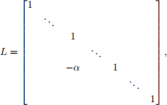 (1)
(1)
where the“α”is in the ith row and jth column with i > j . Let Eij ∈ Rn ×n be the (i,j)th standard basis matrix for Rn ×n , whose (p,q)th component is given by:
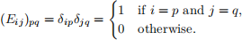 (2)
(2)
The matrix L can be written:
L = I − αEij , (3)
where I ∈ Rn ×n is the n × n identity matrix.
1. Compute the product of two standard basis matrices, Eij ∈ Rm ×p and E![]() , for each choice of i,j,k ,
, for each choice of i,j,k ,
and l . (Hint : there are two cases. Eij Ekl = 0, or Eij Ekl is another standard basis matrix.)
2. We know from class that L−1 = I + αEij . Prove this explicitly by multiplying out LL−1 .
3. Let j be such that 1 ≤ j < n, and let Li = I − ℓij Eij for i such that j < i ≤ n. Compute Tj = Ln Ln −1 ··· Lj+1 . Write Tj in component form (i.e., like in (1)) and in matrix form. Does the order we multiply the Li’s together matter?
4. Recall from class that—assuming we do not need to do any pivoting—we can successively zero out the
columns of a matrix A ∈ Rn ×n by multiplying on the left with matrices T1 ,T2 , . . . ,Tn −1, which has
the effect of transforming A into an upper-triangular matrix U (i.e., we form Tn −1Tn −2 ··· T1 A = U).
Show that L = T![]() 1 T
1 T![]() T
T![]() 1 is a unit lower triangular matrix with strictly lower-triangular entries
1 is a unit lower triangular matrix with strictly lower-triangular entries
given by Lij = ℓij .
Problem 2. (Partial pivoting.) We can incorporate row swaps to minimize the accumulated floating-point error and avoid dividing by zero when computing the LU decomposition using the algorithm described in class and alluded to in the previous problem. There are many strategies for doing this—a simple and effective one is called “partial pivoting”. The algorithm is a simple modification of what we’ve done so far:
Let ![]() (j) be the partially upper triangularized version of A after applying T1 , . . . ,Tj −1 . Before applying Tj , use a row swap to move the row of
(j) be the partially upper triangularized version of A after applying T1 , . . . ,Tj −1 . Before applying Tj , use a row swap to move the row of ![]() (j) taken from among the jth through nth rows for which |
(j) taken from among the jth through nth rows for which |![]()
![]() j(j)) | is largest into the jth row.
j(j)) | is largest into the jth row.
If we denote the row swap associated with Tj by Pj , then Pj is a permutation matrix that swaps two rows at row j or below (e.g., P1 can swap any of the rows of A, P2 can swap any two rows of ![]() (1) except the first row, etc.). Altogether, after eliminating each column of A, we get:
(1) except the first row, etc.). Altogether, after eliminating each column of A, we get:
Tn Pn Tn −1Pn −1 ··· T1 P1 A = U. (4)
This presents a slight problem—we have row swap permutations interleaved with the Tj matrices, so there is not an immediate path to collecting the Tj ’s to get our LU decomposition. However, all is not lost:
1. Let j be such that 1 ≤ j < n. Prove that there exists another “T” matrix ![]() j such that Pj+1Tj =
j such that Pj+1Tj = ![]() j Pj+1 . Carefully explain how the entries of
j Pj+1 . Carefully explain how the entries of ![]() j relate to Tj . (Hint: for a fixed j, we are not considering all possible row swap permutations P . There are some which are excluded from consideration, based on our description of the algorithm above.)
j relate to Tj . (Hint: for a fixed j, we are not considering all possible row swap permutations P . There are some which are excluded from consideration, based on our description of the algorithm above.)
2. Use the previous part to show that we can obtain an LU decomposition of the form PA = LU from
(4). (Hint: use the fact that the product of two permutation matrices is a permutation matrix. You will also need to use some of the tools you developed in Problem 1.)
Problem 3. Here is some pseudocode for computing the LU decomposition using partial pivoting:
U = A
L = I
P = I
for j = 1, ..., n - 1:
let i such that 1 <= i <= k be the index which maximizes |u[i, j] |
swap U[j, j:n] and U[i, j:n]
swap L[j, 1:j-1] and L[i, 1:j-1]
swap P[j, :] and P[i, :]
for k = j + 1, ..., n:
L[k, j] = U[k, j]/U[j, j]
U[k, j:n] = U[k, j:n] - L[k, j]*U[j, j:n]
where, e.g., the notation “j:n” means the indices j through n inclusive.
Once you have formed the LU decomposition PA = LU , you can solve the linear system Ax = b by first multiplying on the left with P to get PAx = Pb. Substituting LU for PA gives LUx = Pb. Moving L and U to the other side gives x = U −1L−1Pb. So, to compute the solution, we permute b using P , and then applying L−1 followed by U −1 . Multiplying with L−1 is equivalent to solving the system Ly = c for y . Since L is lower-triangular, this can be done efficiently using “forward substitution” in O (n2 ) time. Likewise, multiplying with U −1 can be carried out in O (n2 ) time using “backward substitution”. Altogether, once the LU decomposition has been determined, solving a linear system takes O(n2 ) time total.
1. Give an argument based on the pseudocode above that the asymptotic complexity of building the LU decomposition is O (n3 ).
2. Program this algorithm in Python.
3. Find an efficient way to solve systems of the form Ly = c and Uz = d. You should assume that L is unit lower-triangular and that U is not. Program these algorithms in Python.
4. To test and evaluate your algorithm, you will generate random linear systems to solve. For a given n, use np.random.randn(n, n) to generate a random matrix A, and np.random.randn(n) to generate a ran- dom right-hand side b. As a groundtruth, you can use scipy.linalg.lu, scipy.solve.triangular to
compute the LU decomposition and to do forward and backward substitution. For n = 10, 30, 100, 300, 1000, 3000,
and 10000, generate a random system, solve it using your code and the equivalent SciPy version, and time how long it takes to 1) compute the LU decomposition and 2) solve a linear system using both approaches (do this using Python’s time module). Use matplotlib to make a loglog plot with n on the x-axis and the CPU time on the y axis. Write down your observations.
2023-03-06