Marks achieved in this assignment will contribute towards 50% of the final module mark. For this assignment, you have been divided into groups of 4 or 5 students and the group allocations can be found within the assessment tab on the ELE page. Within a group, you are required to conduct an analysis using Generalized Additive Models  (GAMs) and write a report detailing your analyses, results and present a conclusion. A substantial proportion of the marks are allocated to independent learning, specifically in the use and understanding of GAMs that goes beyond the scope of what was taught in the module.  The project is designed to assess your knowledge obtained from the taught aspect of the module, as well as your ability to learn new material.

Deadline:  Noon (12pm), on 20th March 2022.

Each member of the group should submit one identical pdf via eBART containing your report - it should be written up using a professional word processing software (e.g. LaTeX, R Markdown, or Word). Your report is expected to be concise, well structured and well presented. It should comprise at most four sides of text and should have no more than six figures and/or three tables. Figures, tables or R code are not included in the page limit. You must use A4 paper and a font size of at least 11 points, while lines must be single spaced. No credit will be awarded to additional pages of text. Ensure all figures have appropriate titles, axes and captions. Commented R code (e.g. ‘model  <-  glm( . . .)’) and the outcomes/plots should not form part of your report but should be included as appendices at the end.

There are 100 marks in total, and a brief outline of the marking criteria is given below with approximate marks:

●  [ 15 marks] Understanding and exploration of both the problem and the data.

●  [ 10 marks] Thoroughness and rigour, e.g. clear mathematical description of models.

●  [25 marks] Clear exposition of the steps you took in model fitting and exposition of a final model.

●  [20 marks] Clear presentation and interpretation of results.

●  [ 10 marks] Critical review of the analysis.

●  [20 marks] Clarity and conciseness in writing and tidy presentation of R code and associated plots.

You are expected to work within your group and as a team to conduct the analysis and write the report. I do

not expect every group member to contribute to everything, you should maximise efficiency by working out each others strengths and divide the work out effectively. You will be marked as a group and thus receive the same mark.  You should not work with other groups - strict disciplinary action will be taken for any

plagiarism. Late submissions will also be penalised according the University’s late submission policy.           The data required for this assignment datasets_project .RData can be downloaded from the ELE page and loaded into R using the load() function.

Quantifying spatio-temporal risk from TB in Brazil

You are required to conduct an analysis of tuberculosis (TB) data originating from Brazil, using Generalized Additive Models (GAMs).  Brazil is divided into 557 administrative microregions and the available data

comprises of counts of TB cases in each microregion for each of the years  2012-2014.   The R workspace

datasets_project .RData contains the relevant data set in the form of a dataframe TBdata, which contains the following variables:

1.  Indigenous: proportion of indigenous population (the higher the number, the more the indigenous population) in each microregion;

2.  Illiteracy: a continuous measure of illiteracy levels per microregion, the higher the number the more the illiteracy;

3.  Urbanisation:  the rate of urbanisation of a microregion;

4.  Density:  dwelling density (average dwellers per room) in each microregion;

5.  Poverty: a continuous measure of poverty in each microregion (the higher the number, the higher the poverty levels);

6.  Poor  Sanitation: a continuous indicator of sanitation levels in each microregion (the higher the num- ber the poorer the sanitation);

7.  Unemployment:  unemployment levels in each microregion (high values indicate more unemployment);

8. Timeliness:  timeliness of notification, the average amount of time between diagnosing a TB case and reporting it to the health system - this is a proxy measure for the amount of resources in each microregion.

9.  Year: The year (2012–2014);

10.  TB: The number of TB cases in each microregion for the corresponding year;

11.  Population:  The number of people living in each microregion and year;

12.  Region:  A unique ID number to distinguish the 557 regions;

13.  lon:  the longitude of the centroid of the microregion;

14.  lat: the latitude of the centroid of the microregion;

The aim of this project is to use this data set to quantify TB risk across Brazil over the 3 years, where risk is defined as the rate of TB cases per unit population. The health authorities would like to know whether any of the socio-economic covariates (1–8 above) are significantly affecting the rate of TB per unit population, and if so, in what way. In addition, they would like to understand the a) spatial, b) temporal, and c) spatio-temporal structure of any systematic (structured) risk that is not explained by the covariates. The health authorities want to allocate resources for hospitals to cope with the TB cases, so they would like to know if there are regions where the rate of TB per unit population is high and where you would recommend allocating these

resources.

You are expected to use the GAM framework to analyse the data and thus attempt to answer the questions above. You should find chapter 7 of Wood (2017) useful, as well as the R help file on gam .models (obtained by typing ?gam .models in R, after having loaded the library mgcv).

Note, that datasets_project .RData contains shapefiles brasil_micro and a function plot .map. The latter

uses the former to produce a map of Brazil to plot a vector a values. You may find this useful when exploring the data and presenting the results. Specifically, the function plot.map takes the following arguments:

●  x: a vector of 557 values in the order given in TBdata (one for each microregion) to be plotted;

●  n .levels: number of categories that the range of x will be divided into, to produce the colour scheme. These are calculated as equidistant empirical quantiles, default is 4;

●  main:  a character string to be used as a title on the plot.

●  cex: a number used to manipulate the size of the legend, default is 1.

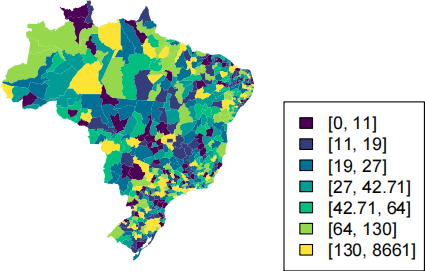
You can of course edit this function as you see fit, or not use the function at all. As an example demonstrating its use, the figure below shows the TB counts in each microregion for the year 2014, using:

# Loading  packages

library(fields)

library(maps)

References

Wood, S. N. (2017). Generalized Additive Models: An Introduction with R (2nd ed.). CRC Press.