Midterm 1 for STAT 4363
Hello, dear friend, you can consult us at any time if you have any questions, add WeChat: daixieit
Midterm 1 for STAT 4363
1. (15 points) Generate 500 observations from each of these autoregressions:
Xt = 0.9Xt − 1 + Ut ,
Yt = −0.9Yt − 1 + Vt ,
where the error terms Ut and Vt are independent white noise series following N(0, 1). You may use the R functions gen .arma .wge() or arima .sim(). Describe the characteristics of these two simulated time series Xt and Yt based on their plots.
2. (15 points) Consider the LakeHuron time series from the datasets package in R. This series Xt has annual measurements of the depth of Lake Huron (in feet) from 1875-1972.
a. Obtain the autocorrelation (ACF) plot of Lake Huron series for the years 1875-1923, and the ACF of the Lake Huron series for the years 1924-1972. Create a panel plot with these two ACF plots.
b. By looking at the panel plot from part a, comment whether the Lake Huron time series from 1875-1972 is stationary.
3. (15 points) Consider co2 time series from the datasets package in R. This series Xt has monthly atmospheric CO2 concentration, measured in ppm, from 1959 to 1997.
a. Apply a Lowess smoother with span choices 0.01, 0.02, 0.03, 0.04. Create a panel plot containing 4 plots, with each plot containing the original and smoothed series at the corresponding span choice.
b. Apply additive or multiplicative seasonal model (you decide and comment on your choice) to this time series using the decompose() function in R.
c. Plot the noise/random component obtained in part c, and also plot its ACF. Comment whether this noise time series behaves like a white noise time series.
4. (15 points) From the FRED website, access the monthly data set containing the housing inventory’s median days on market between 07/2016-01/2023. The data are available at https://fred.stlouisfed.org/series/MEDDAYONMARUS
a. Download the csv. File HIMD.csv to a location of choice.
b. Read the .csv file using the commands HIMD.read = read.csv(file.choose(), header=TRUE)
c. Make a plot of this time series with the dates showing up on the x-axis.
d. Describe the behavior of the data (cyclic, seasonal, trend, wandering,...)
e. Consider a subset of this time series during the period 07/2016-12/2019. Is an additive or multi- plicative seasonal model more suitable (No need to fit the seasonal model)? Explain your choice.
5. (10 points) The figure below includes plots of three time series, each of length 500, along with their sample ACF plots. Which of these three time series behaves like a white noise? Explain. Note that the x-axis of the ACF plots begin only at lag 1.
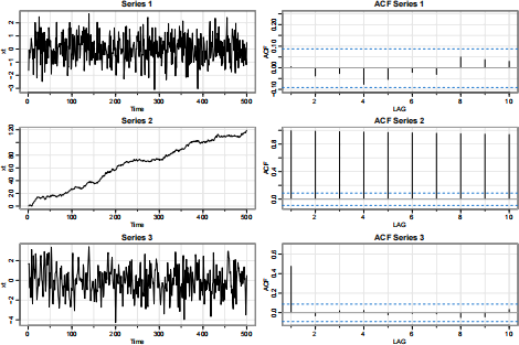
Figure 1: The x-axis in the sample ACF plots starts at lag 1.
2023-03-02