Business Intelligence Techniques and Applications Sample Final Exam Winter 2022
Hello, dear friend, you can consult us at any time if you have any questions, add WeChat: daixieit
Business Intelligence Techniques and Applications
Sample Final Exam
Winter 2022
1. (6 points totalff 1 point each) True or False. If the answer is True, you need to indicate this. If the answer is False, you need to indicate this and give the correct statement.
(a) A random forest adopts two-way randomization to increase the correlations between differ- ent individual trees.
(b) It is a good common practice to set the model parameters to directly maximize the accu- racy on the testing set.
(c) The out-of-sample R2 of a regression model may be 1.5.
(d) The principal component analysis (PCA) decreases the dimension of the feature space.
(e) The exclusion restriction assumption for instrumental variable analysis can be tested with data.
(f) Directly regressing future incomes on the length of education will provide an overestimate for the causal effect of education on earning.
2. (8 points, 2 points each) Short Answers
(a) Which of the following four algorithms do you recommend to normalize the features before running them: (i) k-nearest neighbors, (ii) decision trees, (iii) principal component analysis, and (iv) k-means?
(b) If the data sample for a classification model is very imbalanced (e.g., there are a lot of negative outcomes but very few positive outcomes), is overall accuracy or ROC-AUC a better metric to evaluate the model?
(c) For a randomized experiment, does the conditional independence assumption (CIA) hold?
(d) What is the name of the Instructor of this course? What is the name of the TA of this course?
3. (4 points total) Data Analysis Basics
The data set polling.csv contains the polling data for United States Presidential Election in 2004, 2008 and 2012. The variables are listed as follows:
• State: Name of state
• Year: Election year (2004, 2008, 2012)
• Rasmussen and SurveyUSA: Voters who said they were likely to vote Republican % - voters who said they were likely to vote Democrat %, from two major polling data resources, Rasmussen and SurveyUSA.
• DiffCount: Number of polls that predicted a Republican winner in the state - number of polls that predicted a Democratic winner
• PropR: The proportion of all polls that predicted a Republican winner
• Republican: Whether a Republican actually won that state in that particular election year (the label, taking a 1/0-value)
We run the Python code in Figure 1 to load the data and compute metric_1:
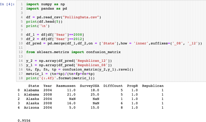
Figure 1: Question 3 Python Code - Part 1
(a) (3 points) For the code in Figure 1, what operation does line 10 of the code perform? What is the data frame df_pred? What is variable metric_1 we evaluate with line 17 and report with line
18 of the code?
(b) (1 point) Then, we run the code in Figure 2. What is the second column of the output (in green box)?
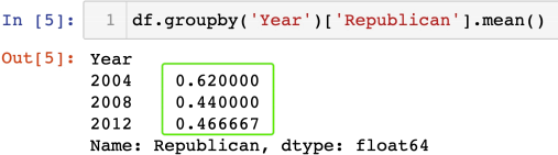
Figure 2: Question 3 Python Code - Part 2
4. (6 points total) Boston Housing Price Prediction
We consider the Boston housing price data set which contains the following set of variables:
• CRIM : Per capita crime rate;
• ZN : How much of the land is zoned for large residential properties;
• INDUS: Proportion of the area used for industry;
• CHAS: Binary variable, 1 if a census tract is next to the Charles River;
• NOX: Concentration of nitrous oxides in the air, a measure of air pollution;
• RM : Average number of rooms per dwelling;
• AGE: Proportion of owner-occupied units built before 1940;
• DIS: Measure of how far the tract is from centers of employment in Boston;
• RAD: Measure of closeness to important highways;
• TAX: Property tax per 10,000 dollars of value;
• PTRATIO: Pupil to teacher ratio by town;
• TRACT : Index of the tract;
• lstat: The percentage of homeowners in the neighborhood considered ”lower class” (working poor);
• MEDV : Median value of owner-occupied homes, measured in thousands of dollars.
(a) (1 point) Consider the Python code in Figure 3. (i) In Line 4 of the code, we create a new variable named HighPrice. What is the interpretation of the variable HighPrice? (ii) Explain the purpose of the last line of the code in Figure 3.
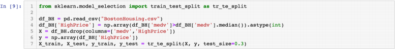
Figure 3: Question 4(a)
(b) (1 point) We next run the Python code in Figure 4. What is the model built in Figure 4?

Figure 4: Question 4(b)
(c) (2 points) The code in Figure 5 produces the confusion matrix therein. Is it an in-sample measure or an out-of-sample measure? What is the overall accuracy of the model? If we change the classifier by adjusting t to 0.7, please give the possible range for the false-positive rate and the false-negative rate of the new classifier.
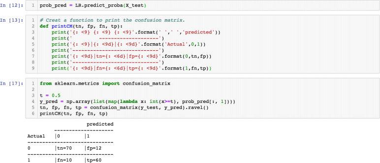
Figure 5: Question 4(c)
(d) (2 points) The final pieces of code we run for the analysis is given in Figure 6. How does the metric AUC relate to the plot in Figure 6? If we change the parameter t in part (c) to t = 0.3, how will AUC change?
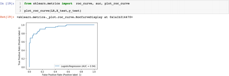
Figure 6: Question 4(d)
5. (6 points total) Bias-Variance Trade-off and Gradient Boosting Tree
(a) (2 points) For a gradient boosting tree, explain the relationship between generalization er- ror GE and the value of K , i.e., the total number of individual trees. Please indicate which region is for high bias and which is for high variance. You may use a graph, with GE as the y−axis and K as the x−axis, to answer this question.
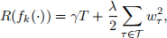
(b) (2 points) Regularization is a standard approach to balance the bias-variance trade-off and address over-fitting. In gradient boosting tree, the usual format of the regularization term is, for each individual tree fk(·),
 (1)
(1)
where T is the total number of leaves for the individual tree fˆk(·), T is the set of all leaves (so |T| = T), and wτ is the weight (i.e., predicted outcome) of leaf τ . What implication(s) would a large γ or a large λ have on the fitted model?
(c) (2 points) Following the code in Question 4, we continue to run the code in Figure 7. What has been done with the code in Figure 7?
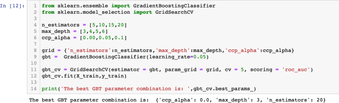
Figure 7: Question 5(c)
|
X |
-10 |
-8 |
-3 |
0 |
10 |
6. (4 points total) Clustering.
(a) (3 points) Consider a data set D as shown in Table 1. Perform the k−means algorithm for k = 2 and the initial centers are C1 = −15 and C2 = 10. What are the two clusters produced by the k-means algorithm? Please provide the center of each cluster.
(b) (1 point) For a clustering model, if all the features are dummy/binary variables, do we need to standardize the features?
|
Group Sample Size Mean Health Status Std Error |
|||
|
Hospital No Hospital |
7774 90049 |
3.21 3.93 |
0.014 0.003 |
|
|
|||
|
Subject |
Wi |
Yi |
Yi(1) |
Yi(0) |
Treatment Effect |
|
1 |
1 |
8 |
|
|
|
|
2 |
0 |
2 |
|
|
|
|
3 |
0 |
4 |
|
|
|
|
4 |
1 |
6 |
|
|
|
|
5 |
0 |
6 |
|
|
|
|
6 |
1 |
4 |
|
|
|
7. (6 points) Potential Outcomes Model and Randomized Experiments
Note: For Question 7 and Question 8, we assume SUTVA holds.
(a) (2 points) Table 2 summarizes the National Health Interview Survey results, where the Health Status refers to the average health condition of a patient when s/he is discharged from a hospital. 1 refers to poor health; 5 refers to excellent health. Based on the survey results, someone argues that, because 3.21<3.93 and it is statistically significant, a hospital makes patients’health poorer. What is wrong with this argument?
(b) (2 points) Consider a randomized experiment with 6 observations, of which two subjects were randomly assigned to treatment via complete randomization. We use Wi ∈ {0, 1} and Yi (1 for treatment and 0 for control) and the observed outcome for subject i, respectively. We use Yi(0) to denote the potential outcome for subject i if untreated and Yi(1) to denote the potential outcome for subject i if treated. Table 3 shows the data observed from this experiment, augmented with columns for potential outcomes and the treatment effect for each subject. Copy Table 3 on your solution paper and fill in all the empty cells in based on the observed information, denoting un- known information with a“?”.
(c) (2 points) Provide an estimate of the average treatment effect based on the data provided in Table 3. Is your estimate unbiased? Why or why not?
8. (4 points) Observational Studies and Instrumental Variables
(a) (2 points) TikTok is considering establishing a new feature that could facilitate the process of searching and connecting to a new friend. The company runs an online randomized experiment to examine the whether users’ adoption of this new feature could improve their satisfac- tion. To do so, TikTok randomly selects a sample of 10,000 users. Within this sample, a random group of users are selected into the treatment group. TikTok sends an encouragement message to each individual in the treatment group. The encouragement message advocates the new feature and encourages the user to adopt it. The rest of the users in the sample are in the control group, to which TikTok sends nothing. TikTok cannot control which user will adopt their new feature, but believes that the adoption of the new feature is positively correlated with receiving the encourage- ment message. Users who are initially more satisfied with TikTok before the experiments will be more likely to adopt the new feature. At the end of the experiment, TikTok conducts a survey that asks each user in the experiment to report his/her satisfaction level of TikTok then. We assume
that each user truthfully reports his/her satisfaction level of TikTok. The data NewFeature.csv has 3 variables:
• Encouragement: An indicator of whether the user has received the encouragement. Encouragement = 1 if the user received the encouragement; Encouragement = 0 if the user did not receive the encouragement.
• Satisfaction: The reported satisfaction level. A higher value means the user is more satisfied.
0 means not satisfied at all; 10 means fully satisfied.
• Adoption: An indicator of whether the user has adopted the new feature. Adoption = 1 if
the user adopted the new feature; Adoption = 0 if the user did not adopt the new feature.
The code used to perform the instrumental variable analysis for the experimental data is provided in Figure 8. Based on the results in Figure 8, provide the estimate for the causal effect of adopting the new feature on user satisfaction. In order for this estimate to be unbiased, we need the strong first stage assumption and the exclusion restriction. Based on the analysis in Figure 8, we know the strong first stage assumption holds. Why? In order for the exclusion restriction assump- tion to hold, what additional assumption do we need?
(b) (2 points) In the first few months of 2021 when COVID-19 vaccination was first introduced to the US, a strange phenomenon was observed: With county-level data, the county infection rate (the number of infection cases divided by the population of the county) was increasing in the vaccination rate (statistically significant), which was contradictory to that, the protection rate of vaccination was about 94% to 95% then (i.e., the infection rate will decrease by a factor of about 95%; or the infection rate of those not vaccinated was about 20 times of the infection rate of those vaccinated). Provide a hypothesis that could reconcile this contradiction. Propose a regression analysis that could validate or dis-validate your hypothesis. What new data do you need for your regression analysis?
Hint: The contradiction discussed above was driven by an omitted variable bias. You may think

about the behavior of the people who chose not to get vaccinated. Another information that you may find useful is, at that time and in the entire US, the total number of infection cases of those vaccinated was 5,814 (out of about 75,000,000, with an infection rate 0.007752%), whereas the total number of the infection cases not vaccinated was 12,000,000 (out of about 225,000,000, with an infection rate 5.33%). Thus, the infection rate of those not vaccinated was about 688 times of the infection rate of those vaccinated.
2023-02-23