MA261 Assignment 2
Hello, dear friend, you can consult us at any time if you have any questions, add WeChat: daixieit
MA261
Assignment 2 (20% of total module mark)
due Thursday 23nd Feburary 2023 at 12pm
Regulations:
● Python is the only computer language to be used in this course
● You are not allowed to use high level Python functions (if not explicitly mentioned), such as diff, int, taylor, polyfit, or ODE solvers or corresponding functions from scipy etc. You can of course use mathematical functions such as exp, ln, and sin and make use of numpy .array.
● In your report, for each question you should add the Python code, and worked-out results, including figures or tables where appropriate. Use either a Python script and a pdf for the report or combine everything in a Jupyter notebook. We need to be able to run your code.
● Output numbers in floating point notation (using for example the npPrint function from the quiz).
● A concisely written report, compiled with clear presentation and well structured coding, will gain marks.
● Do not put your name but put your student identity number on the report.
● The first part of each assignment needs to be done individually by each student.
● For the second part submission in pairs is allowed, in which case one student should submit the second part and both need to indicate at the top of the their pdf for the first part the student id of their partner. Both will then receive the same mark for the second part of the assignment.
Q 1.1. [2/20]
Consider the following chemical reaction network
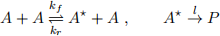
where A is some molecule and P the product of the reaction. A★ is called a reaction intermediate. Assume given initial conditions A0, A0(★), P0 .
(1) Derive the system of ODEs for A, A★ , P modelling the above reaction network. Using a conservative quantity derive a system of ODEs for only A, P .
(2) A typical model simplification approach is to make a steady-state approximation in which one assumes that the rate of production of a quantity equals the rate of consumption so that its time derivative is zero. In the above reaction it is often reasonable to make this assumption for A★ .
Using the steady-state approximation that A★ does not change in time, derive a new system of ODEs involving only A, P .
Q 1.2. [3/20]
Consider a two stage explicit RK method given by the Butcher tableau 
where a, γ e [0, 1].
We know that this method will always be first order and to make it second order we need to choose the constants so that x := aγ = ![]() .
.
Instead of optimizing the order, we will now try to optimize the stability of the method. First consider the linear case y\ = λy with real valued λ < 0. We are looking to maximize h0 = h0 (a, γ) so that the method is stable (i.e., yn → 0 for n → o) for h < ![]() .
.
(1) Compute the stability bound h0 and show that it only depends on the product x = aγ of the two free parameters (as we have seen the order does).
(2) Find the value xopt for x for which h0 is largest so that lynl remains bounded. Explanation: if you take x slightly above xopt and h slightly below h0 then lynl → 0 as originally required. Taking x = xopt is not quite enough - in a sense xopt is an infimum and not a minimum. That makes the question slightly more difficult to formulate than I realized. That is why I am now only asking for boundedness of lynl.
If you want to you can make the following quite easy calculation: for any ε > 0 take x = xopt(1 + ε) then the method will satisfy yn → 0 for h < ![]() . But as I said you don’t need to show this.
. But as I said you don’t need to show this.
(3) Consider the same two stage explicit Runge-Kutta method but now we take λ = αi with real α ![]() 0. For which choices of x = aγ is there a positive h0 > 0 so that for h <
0. For which choices of x = aγ is there a positive h0 > 0 so that for h < ![]() the method is stable, i.e., satisfies lynl < ly0 l for all n?
the method is stable, i.e., satisfies lynl < ly0 l for all n?
Extra: You don’t have to write down the answers to the following follow on questions: the only one stage explicit Runge-Kutta method is the Forward Euler method. By adding a second explicit stage we have doubled the computation cost (roughly speaking). By chosing x = xopt, how much larger can we take the time step compared with the Forward Euler method - is it worth doing? Is there any h0 for the Forward Euler method for which the solution remain bounded in the case λ = iα - again do we gain by adding a step?
Q 1.3. [5/20]
Consider a Hamiltonian H(x, p) and the induced Hamiltonian system
x\ = ∂pH(x, p) , p\ = ·∂xH(x, p) .
To simplify things we will assume that x, p are scalar.
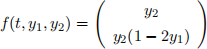
For an approximation (xn, pn) define Hn := H(xn, pn). We would like to find approxima- tions with Hn = H0, i.e., the method conserves the Hamiltonian in time. We will study three methods. For the first two we will only prove results in the case that the Hamiltonian is of the form
(*) 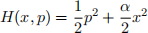
with some positive constant α . We will show that the third method exactly conserves a general Hamiltonian in each step.
. The first is the Forward Euler method.
. The second is the so called semi-implicit Euler method
(SI-E) xn+1 = xn + h∂pH(xn, pn) , pn+1 = pn · h∂xH(xn+1, pn) .
As you can see this is a very simple modification of the standard Forward Euler method for the case of Hamiltonian systems. This is a type of split method - which
in fact is explicit in spite of the name.
. The third method is fully implicit and also split:
(FI-Method) 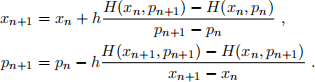
Make sure you understand why this is a reaonable approximation of the Hamil- tonian system...
(1) Consider the case of the quadratic Hamiltonian (*) and the approximation (xn, pn) to the Hamiltonian system from the Forward Euler method.
We have already seen simulations in the lecture that indicate that in this case the value of the Hamiltonian increases in each time step, i.e., Hn+1 > Hn .
Prove that this is the case by showing that Hn = (1 + αh2 )n H0 .
(2) Consider now the semi-implicit Euler method (SI-E). Show that when applying this method to the quadratic Hamiltonian (*) the method can be rewritten as
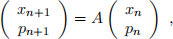
with a suitable matrix A.
Note: In fact the method conserves a “perturbed Hamiltonian“ Eh(x, p) := H(x, p) · h ![]() px. One can use this to show that Hn stays O(h) close to H0 but we will not do that in the lecture.
px. One can use this to show that Hn stays O(h) close to H0 but we will not do that in the lecture.
(3) Consider now a general Hamiltonian and the approximation given by the fully implicit method (FI-Method). Making the assumption that pn+1 ![]() pn and xn+1
pn and xn+1 ![]() xn, show that Hn = H0 for all n.
xn, show that Hn = H0 for all n.
PART 2
Hand in one program listing which covers all the questions given below in a single scrip- t/notebook reusing as much as possible. Avoid any code duplications (or explain why you decide to duplicate some part of the code).
Important: In your brief discussion of your result (a paragraph with a plot or a table is sufficient) refer back to the theoretical results discussed in the lecture or from assignments.
Q 2.0. [see online quiz on moodle]
Implement the following functions and test them individually. Take a look at the quiz questions which also include some tests and more detail on the function signature to use. After the quiz closes you can use the provided solutions if you encountered problems implementing the required functions.
You do not need to include any testing you did of these method in the report.
(1) Write a function that computes the root of a given function F : Rm → Rm . The function F and its Jacobian should be passed to the function using function han- dles. In addition the function requires an initial guess x0 , a tolerance ε, and a maximum number of iterations K to perform before giving up. The iteration stops with the kth iterate xk if either lF (xk)l < ε or k = K .
The function should return the final approximation xk to the root and the number of steps k used. So if the returned number of steps equals the maximum number of iterations provided as parameters, i.e., k = K then the Newton method failed to converge and any calling function should handle that case, e.g., terminate with an error.
(2) Write a function that computes a single step of the backward Euler method
yn+1 = yn + hf(tn+1, yn+1)
given h, tn e R and yn e Rm and a general vector valued function f which should be provided together with its Jacobian with respect to y . Use Newton’s method to solve the nonlinear problem.
Q 2.1. [1/20]
Implement the Crank-Nicholson method given by
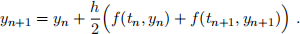
We have seen in the seminar that this method converges with second order.
Repeat the first experiment from the first assignment comparing the forward Euler method, the backward Euler method, the method Q11 from assignment 1, and the Crank-Nicholson method.
So you should compute the maximum errors and EOCs for all four methods for the ODE with right hand side
for t e [0, 10] and y0 = (2, ·2)T using the time step sequence hi = ![]() for i = 0, . . . , 9 using N0 = 25.
for i = 0, . . . , 9 using N0 = 25.
Q 2.2 (you can discuss this together with Q2.3 and Q2.4 if you want). [2/20]
Consider the Hamiltonian system for y = (x, p) induced by the Hamiltonian for a non- linear mass-spring system H(x, p) = ![]() p2 + V (x) where the potential is given by
p2 + V (x) where the potential is given by
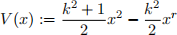
with positive constants k, r .
For r = 2 the Hamiltonian system is a harmonic oscillator and since it’s linear you can easily find the exact solution. For r = 4 the system is know as Duffy equation and the exact solution for this problem is given by the elliptic Jacobi functions which are available from scipy .special .ellipj. For the initial conditions y0 = (0, 1) the solution is:
|
from scipy . special import ellipj def Y ( t ): sn , cn , dn , _ = ellipj (t , k * k ) return array ([ sn , cn * dn ]) # ( x ( t ) ,p ( t )) |
Do the following experiments for both r = 2 and r = 4. Use k = 0.8, y0 = (0, 1) as initial conditions, and simulate up to T = 40: compare errors and EOCs for the two second order methods (Q11 and Crank-Nicholson) and the backward Euler method using the time step sequence hi = ![]() 2一i for i = 0, . . . , 10.
2一i for i = 0, . . . , 10.
Add plots of the trajectories in phase space for i = 0, 1 for all three methods.
Q 2.3. [3/20]
Implement the semi-implicit Euler method discussed in Q1.3 above: You can restrict your implementation to scalar x, p and the case of a Hamiltonian of the form H(x, p) = ![]() p2 + V (x). But of course you can also do the general case.
p2 + V (x). But of course you can also do the general case.
Repeat the experiments from Q1.2. How does the new method compare to the others? Which rate of convergence do you think the new method has?
In addition to the errors also discuss the relative error in the Hamiltonian for all methods,
i.e., study the sequence (hi, Eh(Ham)) with Eh(Ham) := maxn ![]() y(一)
y(一)![]()
Hint: You should be able to write a function mapping yn = (xn, pn) to yn+1 = (xn+1, pn+1) that you can use as stepper in your code. It is sufficient to implement this function for y = (x, p) with scalar x, p but feel free to consider the general case. After doing that you should be able to use the code from Q2.2.
Q 2.4 (this question is perhaps a bit harder...) [4/20]
Implement the fully implicit method from Q1.3. Optimize the implementation for the case of a Hamiltonian of the form H(x, p) = ![]() p2 + V (x). To optimize the implementation first rewrite the method in the form
p2 + V (x). To optimize the implementation first rewrite the method in the form
xn+1 = xn + hϕx(xn, pn, xn+1; h) , pn+1 = pn + hϕp(xn, pn, xn+1) ,
using that H(x, p) = ![]() p2 + V (x). Add your formulation to your report... It is okay to implement the method only for scalar x, p.
p2 + V (x). Add your formulation to your report... It is okay to implement the method only for scalar x, p.
Repeat the experiments from Q1.3. How does the new method compare to the others? Which rate of convergence do you think the new method has?
Hint: After you reformulated the method to make use of the special form of the Hamil- tonian, you will need to use Newton’s to compute xn+1 from given (xn, pn). After that step, pn+1 is explicitly computable.
Depending on how you ended up defining ϕx, you might have to put some thought into finding a good initial guess to use for Newton’s method. Explain what you did and why you think that is a good choice for the initial guess. If you couldn’t get it to work, give a short description of what you tried - it might still earn you some marks.
2023-02-21