AMATH 301 – Winter 2023 Homework 5
Hello, dear friend, you can consult us at any time if you have any questions, add WeChat: daixieit
AMATH 301 – Winter 2023
Homework 5
Due: 11:59pm, February 17, 2023.
Instructions for submitting:
● Coding problems are submitted to Gradescope as a python script/Jupyter notebook ( .py or .ipynb file). (If you use Jupyter Notebook, remove all “magic”: the lines that begin with %). You have 8 attempts (separate submissions to Gradescope) for the coding problems.
● Writeup problems are submitted to Gradescope as a single .pdf file that contains text, plots, and code at the end of the file for reference. Put the problems in order and label each writeup problem. When you submit, you must indicate which problem is which on Gradescope (including the code that belongs to the problem). Failure to do so will result in a 10% penalty. . All code used for each problem should be included at the end of that problem in your .pdf file and be marked as part of the problem on Gradescope. Failure to include code will result in a 25% penalty.
Coding problems
1. (This problem goes with Writeup Problem 1 . You may want to work on that problem at the same time as this problem)
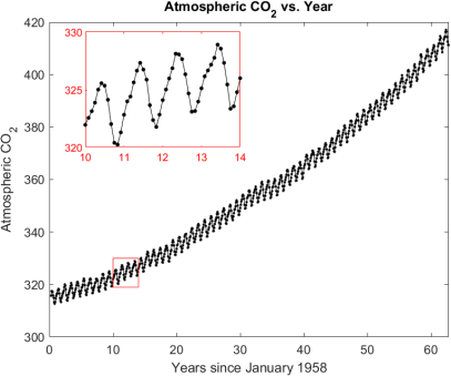
The amount of CO2 in the atmosphere is regularly measured at the Mauna Loa observatory in Hawaii. The file CO2_data .mat (or CO2_data .csv for python), which is included with the homework, contains the monthly averages since March 1958 up until December 20221. A plot of a similar dataset (up until December 2020) is shown on the next page. The data has an overall upward trend as well as seasonal oscillations.
(a) Load this data (CO2_data .mat or CO2_data .csv) into your homework solution file. Be sure that the file CO2_data .mat has been downloaded into the same directory as your script file. You do NOT need to upload this file to the autograder, it has its own copy. CO2_data .mat contains two arrays: CO2 contains the monthly averages and the array year contains the years since January 1958 as a decimal (e.g., March 1958 is 3/12 = 0.25 because it is the third month in 1958).
To make sure that you have loaded in the data correctly, save the array year to the variable A1 and the array CO2 to the variable A2.
(b) It looks like the overall trend of the data might be captured well by using an
exponential fit. We seek a model of the form
y = a + bert .
To do so, create a function that takes the values of a, b, and T as inputs and calculates the sum of squared errors (as we have done in class, without the square root) as output. First, to check that you have defined the error function correctly, save the value of the error your function calculates to the variable A3, using a = 300, b = 30, and T = 0.03.
(c) We can now find the optimal parameters using scipy .optimize .fmin to find the values of a, b, and T that minimize the sum of squared errors (and therefore minimize the root-mean squared error). Use this method to find the best fit curve of the form
y = a + bert . Use the initial guesses of a = 300, b = 30, and T = 0.03. Make an array with 3 elements with the optimal parameters and save this array to the variable A4. You will plot this curve in Writeup Problem 1.
(d) Save the total Sum of Squared Errors for the optimal model to the variable A5. (Hint: you have the parameters now, how do you get the error from those parameters?)
(e) Repeat the above problem using the max error. Save the error for a = 300, b = 30, and T = 0.03 to the variable A6 and the optimal parameters to the variable
A7.
Note: Since this is a hard optimization to solve, scipy needs to evaluate more iterations to find the minimum than the default settings. To fix this, simply
add maxiter=2000 as your third argument to
scipy .optimize .fmin, e.g,
scipy .optimize .fmin([function here], [guess here], maxiter=2000)
(f) The best-fit curves you found match the overall trend well (I recommend plot- ting one or some!), but they still do not capture the seasonal oscillations. In
order to capture the oscillations, we can find a best fit curve of the form y = a + bert + c sin(d(t 一 e)).
Create sum-of-squares error function. To check your error function, Save the error for a = 300, b = 30, r = 0.03, c = 一5, d = 4, and e = 0 to the variable
A8.
(g) We now want to find the optimal parameters for this model. Since this model is similar to the model in part (b), we think that a, b, and c will be similar to what are found there in A4. Because of this, your initial guess for a, b, and r will be the exact values you found for A4 (not output that you copied and pasted). Use c = 一5, d = 4, and e = 0 as initial guesses for the other parameters. You may want to use np .append here. Since this model is different, the resulting a, b, and r found here will be different from the a, b, and r recorded in A4. Note: See the note in part (e). You will again need to increase maxiter. Make an array with 6 elements with the optimal parameters [a, b, r, c, d, e], and save this vector to the variable A9. You will plot this curve in Writeup Problem 1.
(h) Save the total Sum of Squared Errors for this model to the variable A10.
2. Download the file salmon_data .csv included with the homework. Make sure this file is in the same folder as your homework file. This file contains the annual Chinook salmon counts taken at Bonneville on the Columbia river (in the second column) from the years 1938 to 2021 (in the first column)2. In this problem we will fit this data with a curve to predict salmon populations.
(a) Load salmon_data .csv in your solution script. The data has two vectors: year is the year and salmon is the salmon count in the corresponding year.
You do NOT need to upload this file to Gradescope. Your code will be tested using the counts for another species of salmon. Because of this, your code should not have any answers hard-coded in: your code needs to work for whatever data set is provided.
(b) Use polyfit to find the line of best fit (degree 1). Save the coefficients for the polynomial as an array to the variable A11.
(c) Use polyfit to find the best-fit polynomial of degree 3 for this data. Save the coefficients for the polynomial as an array to the variable A12. (Note: you may get a warning here, ignore it.)
2 Data from www .cbr .washington .edu
(d) Use polyfit to find the best-fit polynomial of degree 5 for this data. Save the coefficients for the polynomial as an array to the variable A13. (Note: you may get a warning here, ignore it.)
(e) You now have three models for predicting the number of salmon in a given year: a degree-1 polynomial, a degree-3 polynomial, and a degree-5 polynomial. Call these three polynomials p1 , p3 , and p5 respectively. You will plot these in Writeup Problem 2.
The number of Chinook Salmon in 2022 was 752638. For each of the three polynomials, find the percentage error between what your polynomial predicts is the number of salmon in 2022 and the true number of salmon. In other
words, calculate
err1 = ![]() 63(一)
63(一)![]()
![]() err2 = |p3 (2022) 一 752638| ,
err2 = |p3 (2022) 一 752638| ,
err3 = ![]() 63(一)
63(一)![]()
Create an array with the components
[err1 , err2 , err3].
Save this array to the variable A14. Warning: Make sure that you are evalu- ating pn (2022) using the built-in python function for doing so, otherwise your answer will not be within the Gradescope error tolerance.
Writeup problems
1. (This problem goes with Coding Problem 1 . You may want to work on that problem at the same time as this problem) .
You need to turn in the plot in part(a), the answers to parts (b)&(c), and all of the code used for this problem.
(a) Create a plot that contains the atmospheric CO2 data and your two curves of best fit found using the sum of squared error (A4 and A9) in Coding Problem 1. Make sure to plot with enough resolution to capture the oscillations. Your plot should look similar to the figure in Problem 1, except without the red insert.
i. The data should be plotted as black dots connected by black lines by using the line specification ’-k . ’ . Use markersize = 2.
ii. Your plot should show from t = 0 to t = 65.
iii. The exponential + sinusoidal fit (A9) should be plotted as a blue curve and it should have line thickness 2. You need to plot this curve first before the other curve.
iv. The exponential fit from Coding Problem 1 (c) (A4) should be plotted as a red curve and it should have line thickness 2.
v. Label the x-axis with “Years since January 1958”
vi. Label the y-axis with “Atmospheric CO_2”
vii. Include a legend that does not block the data (northwest is good).
viii. Include a meaningful title.
(b) In Coding Problem 1 you calculated sum of squares error for the two curves (A5 and A10). Record the error for each of the methods and compare the error. Which of the two methods gives smaller error? How can you see that in the plots?
(c) Suppose we wanted to predict the amount of atmospheric CO2 at Mauna Loa for January 2023. Which of the models do you think is more appropriate for this task? You need to justify your answer.
2. (This problem goes with Coding Problem 2. You may want to work on that problem at the same time as this problem)
You need to turn in the plot in part (a), the responses from part(b)-(d), and all of the code used for this problem.
(a) Create a plot of the salmon data from Coding Problem 2 along with the three functions created in that problem, p1 , p3 , and p5 . Your plot should have the following features:
i. The data should be plotted as black circles with black lines in between the circles. You can do this by using the line specification ’-k . ’ .
ii. Your plot should be from 1930 to 2025 on the x-axis and from 100,000 to 1,500,000 on the y-axis.
iii. p1 should be in blue, p3 in red, and p5 in magenta. These lines should have linewidth 2.
iv. Your plot should have a legend that does not block any of the data or curves (northwest is good).
v. Label the x-axis with "Year " and the y-axis with "Number of Salmon".
vi. Include a meaningful title.
(b) What does the slope of the line of best fit tell us about how the population is generally changing over this timeframe?
(c) Of the different polynomials you tried in Problem 1, which gave the most accurate prediction of the 2022 salmon population and which gave the least accurate prediction?
(d) Suppose we want to predict the salmon population in 2050. Rank the three models by which you trust the most for this prediction. Justify your answer by including the values each of these methods predict for the population in
2050.
2023-02-19