闪电代写 -代写CS作业_CS代写_Finance代写_Economic代写_Statistics代写_代码代做_IT代写_加急帮助

Hello, dear friend, you can consult us at any time if you have any questions, add WeChat: daixieit

Chemical kinetics: Decomposition of hydrogen peroxide

INTRODUCTION

In this experiment, you will investigate the kinetics of the decomposition of hydrogen peroxide, H2O2, in the presence of iodide. The chemical equation for the reaction is

2H2O2 (aq) → 2H2O(l) + O2 (g).

The rate of the reaction may be expressed as ∆time , which equals the slope of a plot of PO2 versus time, provided the graph is linear. The rate of the reaction is dependent upon the initial concentration of H2O2 and upon the concentration of iodide, a catalyst added to the aqueous solution. In this experiment the order of the reaction with respect to H2O2 and with respect to I- is to be established. The general expression for the differential rate law is

rate = k[H2O2]m [I-]n .

Taking the log of both sides of this equation leads to

log(rate) = log k + m log[H2O2] + n log[I-].

If [I-] is constant, then a plot of log(rate) versus log[H2O2] is linear with slope = m, the order of the reaction with respect to H2O2 . If [H2O2] is constant, then a plot of log(rate) versus log[I-] is linear with slope = n, the order of the reaction with respect to I- .

In this experiment, the reaction rate is measured as a function of initial molarities. For three trials, the initial molarity of I- is fixed while the initial molarity of H2O2 is varied. For another three trials, the initial molarity of H2O2 is fixed while the initial molarity of I- is varied.

Once the orders of the reaction are known, the value of the rate constant, k, can be obtained from a graph of either rate versus [H2O2]m where the slope = k[I-]n (with [I-] constant) or rate versus [I-]n where the slope = k[H2O2]m (with [H2O2] constant).

For a fixed set of initial molarities, the reaction is to be run at three different temperatures. According

to the Arrhenius equation, ln k = ln A - ,

where Ea is the activation energy. When the initial concentrations are fixed the graph of ln(rate) versus 1/T should yield a straight line with slope equal to -Ea /R.

PROCEDURE

This is apartnership experiment.

Part 1. Preparation for the kinetic study

Step 1. Pressure sensor calibration. Get the atmospheric pressure

reading in the lab. Start the Kinetics program. Make sure the syringe is

disconnected from the pressure sensor. Pull the piston to the 20.0 mL mark.

Keeping the piston at this setting, attach the syringe to the pressure sensor.

Under the Experiment menu click on Calibrate and then on Lab Pro: 1 CH 1: Gas Pressure Sensor.

Remove the check mark in the “One Point Calibration” box and click on

Perform Now. Enter the atmospheric pressure in mmHg into the Reading

1 box, and when the voltage reading stabilizes, click on Keep. Depress the

piston of the syringe to the 10.0 mL mark. Enter the value that is double the atmospheric pressure in mmHg, and when the voltage reading stabilizes, click on Keep and on Done.

Step 2. In a clean 250-mL beaker combine 40. mL of 3.0 M H2O2 with 40. mL of distilled water. Label this diluted solution 1.5 M H2O2 . Then, in a 30-mL beaker, combine 10. mL of the 1.5 M H2O2 solution with 10. mL of distilled water and label this beaker (the label should state the final concentration of H2O2 in this beaker). Finally, fill a clean 250-mL beaker with about 150 mL of 0.10 M KI and indicate the concentration of KI on the beaker. Wear rubber gloves!

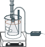
Step 3. Obtain a stopper assembly that consists of a stopper with two valve connections, one Luer-lock connector, and one two-way valve. Connect the stopper to the pressure sensor probe. Fill an 800-mL beaker with 400 mL of room temperature water. Use a digital thermometer to measure the temperature of the water. Leave the thermometer in the beaker to observe any changes in temperature during the reaction. Place the beaker on a magnetic stirrer.

Step 4. Add 10. mL of 0.10 M KI and 15 mL of distilled water to a clean 125-mL

Erlenmeyer flask. Use a 10-mL graduated cylinder for the 0.10 M KI solution and a 25-

mL graduated cylinder for the water. Slide a magnetic stirring bar into the KI solution.

Position the flask such that its contents are submerged in the water in the 800-mL

beaker. Turn on the magnetic stirrer and wait about a minute for the temperature of the

reaction solution in the flask to equilibrate with the bath temperature in the beaker.

Step 5. Measure out exactly 5.0 mL of the 1.5 M H2O2 solution by drawing the solution

into a 5-mL syringe. Make sure the two-way valve in the stopper to the Erlenmeyer flask is closed and then twist the syringe into the top of the valve. Prepare the temperature of the bath close to temperature 25.0oC. Use hot or cold water (get ice if necessary) from the faucet to obtain this temperature in the bath.

Part 2. Kinetic investigations

Step 1. One student should hold the flask and the rubber stopper connected both to the pressure probe and to the filled syringe. The second student should then open the two-way valve, let the first student squirt the measured H2O2 from the syringe into the flask, close the two-way valve, and then immediately click on the Collect button. Since the pressure in the flask increases, hold the stopper firmly in place during each measurement. Between about 30 seconds and about 300 seconds, the plot of pressure versus time should be linear. Monitor the temperature of the bath during the reaction. Record the average temperature during each run in the Data Table.

Note that initially a fast reaction occurs and the solution changes from colorless to yellow. The yellow is due to the formation of I2, as I- is oxidized by H2O2:

H2O2 (aq) + 2I- (aq) → I2 (aq, yellow) + 2OH- (aq).

Step 2. When the line starts to level out with a decrease in slope, click on the Stop button. Turn off the magnetic stirrer. Remove the stopper from the reaction flask before the pressure buildup in the flask pops off the stopper.

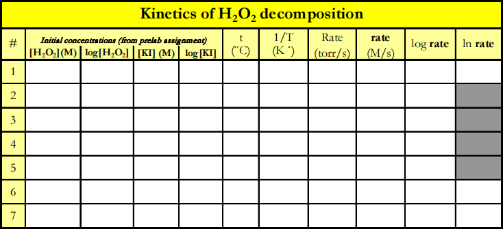
Step 3. Select the linear part of the curve and under the Analyze menu select Linear fit. Double click on the box with the equation and change Displayed Precision to 4 significant figures. In your table, write down the concentration of KI and H2O2 and the rate of reaction (slope of the pressure-versus-time linear fit is the value of the reaction rate in torr/s). Under the Experiment menu click on Store Latest Run.

Step 4. Run six additional trials using basically the same procedure. In two trials, vary the concentration of the KI and in two other trials, vary the concentration of the H2O2 . Finally, vary the temperature. Run each trial in a new clean 125-mL Erlenmeyer flask.

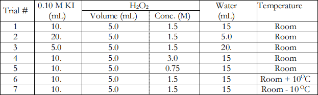
Notes pertaining to the additional trials:

Trials 1-5: Maintain a constant temperature for these trials (25.0 ± 0.5OC).

Trial 4: Use about 10 mL of the 3.0 M H2O2 solution in a small beaker to rinse and to fill the syringe.

Trials 6 and 7: Prepare two baths each with 400 mL of water in an 800-mL beaker. One bath with temperature of about 10oC above and the other of about 10oC below that used in trials 1-5. Use hot or cold water (get ice if necessary) from the faucet to obtain the right temperature. Save the graph with all trials and keep it on file.

CALCULATIONS

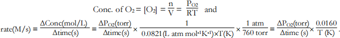
1. Convert the rates of ∆PO2 /∆time to ∆Conc./∆time.

The rate of formation of oxygen is proportional to the slope of the linear fits since, from the ideal gas law, partial pressure is directly proportional to the gas’s concentration:

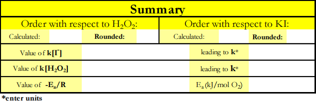
2. Use MS Excel to analyze the results of the first three trials. Calculate log rate and log[KI]. Plot log rate on the vertical axis versus log [KI] on the horizontal axis. Obtain the equation for the slope of the linear graph.

3. Analyze the results of trials 1, 4, and 5. Compute log rate and log[H2O2]. Plot log rate (vertical) versus log[H2O2] (horizontal). Obtain the equation for the slope of the linear graph to three significant figures.

4. Evaluate the rate constant, k, based on the first three trials. In this and next evaluation use the true values of the order with respect to H2O2 (m=1) and with respect to I- (n=1). Plot rate(vertical) versus [KI] (horizontal) to obtain a linear graph. Obtain the equation of the line. Change the format of the displayed equation so the slope contains at least 3 significant figures. From the slope = k[H2O2], compute the value of k. Report it with the proper units.

5. Evaluate the rate constant, k, based upon trials 1, 4, and 5. Plot rate versus [H2O2] to obtain a linear graph. Obtain the equation of the line and the R2 value. From the slope = k[KI], compute the value of

k. Report it with the correct units.

6. Analyze the results of trials 1, 6, and 7. Calculate ln(rate) and 1/T. Plot a graph of ln (rate) versus 1/T. The slope of this linear plot is -Ea /R where R = 8.314 × 10-3 kJ mol-1Kelvin-1 . Evaluate Ea in kJ per mol O2 .