COMP0034 Coursework 1 Visualizations
Hello, dear friend, you can consult us at any time if you have any questions, add WeChat: daixieit
COMP0034 Coursework 1
3. Visualizations
This section walks through the design and its evaluation of each visualization present in the
![]() dashboard. The main references used as sources of information on data visualisation chart
dashboard. The main references used as sources of information on data visualisation chart
types and design considerations are:
1. Interactive Chart Chooser by Depict Data Studio:https://depictdatastudio.com/charts/
2. The Data Visualisation Catalogue developed by Severino Ribecca: https://datavizcatalogue.com/index.html
3. Towards Data Science A Medium publication sharing concepts, ideas and codes: https://towardsdatascience.com/
4. CHARTIO Data Visualization Tutorials:https://chartio.com/learn/tutorials/
5. Efective Data Visualization: The Right Chart for the Right Data . Book by Stephanie Evergreen. (2016).
6. Data Visualization: A Practical Introduction . Book by Kieran Healy and Kieran Joseph Healy. (2018).
7. The Functional Art: An Introduction to Information Graphics and Visualization . Book by Alberto Cairo. (2011).
3.1 Latest Pollutant Concentration Measurements
3.1.1 Questions the visualisation is intended to address
1. What are the most recent measurements of key air pollutant levels (NO2 and PM2.5) in Westminster?
2. What is the current air pollution level?
3. Are the concentrations below the limits above which they may pose some health risks to sensitive populations?
3.1.2 Target audience
![]() At-risk individuals, including people with lung or heart problems, people with asthma and
At-risk individuals, including people with lung or heart problems, people with asthma and
older people living in the area. They may follow appropriate health recommendations and adjust their plans based on the current air quality category. e.g., If air quality is bad (high pollutant levels) elderly people and those with cardiovascular diseases may want to reduce strenuous physical outdoors activity, and people with asthma will make sure that they take their reliever inhaler with them if they go for a walk.
![]() Athletes, such as people who want to go for a run outside, exercise in a park, or some
Athletes, such as people who want to go for a run outside, exercise in a park, or some
other sort of outdoor training. e.g., if the current air quality is bad, they may want to reduce strenuous physical exertion, or go for a run at a later time when the levels of pollutants get smaller.
![]() Parents of young children, depending on the current air quality, may decide whether they
Parents of young children, depending on the current air quality, may decide whether they
want to go play outdoors with their kids now or later. Young children are more vulnerable to air pollutants, and overexposure may lead to development of respiratory diseases.
![]() Pregnant women may decide to go for a walk or not depending on air quality, as both
Pregnant women may decide to go for a walk or not depending on air quality, as both
them and their babies are susceptible to harmful air pollutants.
![]() General public (i.e., all others). Although they may not be considered as ‘at-risk’ group,
General public (i.e., all others). Although they may not be considered as ‘at-risk’ group,
they may still be interested in current air quality, for whatever reasons, and adjust their plans accordingly.
![]() Outdoor workers and their employer. Following the Health and Safety at Work etc. Act
Outdoor workers and their employer. Following the Health and Safety at Work etc. Act
1974, employers may want to limit the outdoor activities of their employees as part of their work if the air quality is bad.
3.1.3 Data
This visualization requires latest measurements of key air pollutants’ (NO2 and PM2.5), obtained from the OpenAQ API.
3.1.4 Chart type
Latest measurements can be conveniently visualized using separate gauges. Angular gauge charts, also called radial gauge charts or simply gauges, are a good way to visualize a single value and are often used to illustrate key indicators.
3.1.5 Design
Each gauge will consist of a circular arc, which displays a single value of pollutant concentration in the form of a shaded bar inside of the arc, allowing to estimate its level on a scale of possible values.
Important parts of each chart include:
![]() A short title, that tells the quantity being shown, and the units of measurement, e.g.,
A short title, that tells the quantity being shown, and the units of measurement, e.g.,
NO2 Concentration (µg/m3).
![]() The actual value, shown in the free space in the middle of the gauge, that gives a numeric
The actual value, shown in the free space in the middle of the gauge, that gives a numeric
representation of the value to accompany the visual representation.
![]() Axis ticks representing the scale of possible values
Axis ticks representing the scale of possible values
![]() Steps that are shown as shading inside the radial arc. Those are linked to the air pollution
Steps that are shown as shading inside the radial arc. Those are linked to the air pollution
banding based on the DAQI.
![]() The difference of the current value and the previous value, i.e., the change in
The difference of the current value and the previous value, i.e., the change in
concentration.
![]() A limit concentration (from EU air quality standards), that is a threshold used to
A limit concentration (from EU air quality standards), that is a threshold used to
determine boundaries that visually alert the person looking at the chart if the value cross a defined threshold.
![]() The date and time of last update, to notify the viewer of how recent the displayed value is.
The date and time of last update, to notify the viewer of how recent the displayed value is.
Angular gauge charts are in principle very intuitive, and hence are appropriate for all audiences. They are very space-efficient and combine four pieces of important information in one visualization:
The actual value of pollutant concentration.
Its level on the scale of possible values, i.e., how small, or large it is.
The air pollution level (band) it falls into.
The change in value compared to the previous one.
How does it compare to the limit concentration.
How recent is it.
This makes it a very powerful visualization that is easy to understand and interpret.
3.1.6 Visual aspects
To be effective, these charts need to be simplistic, and the colour should be appealing and not distracting. The shaded bar inside the arc should be clearly visible and have a good contrast. Axis ticks must be small and light to avoid distraction. The shaded inside the arc will representing the DAQI, and its four air pollution level bands. Hence, it will have ten intervals. Those that fall under the ‘Low’ band (Index 1-3) will be coloured in shades of green , from light green to dark green. Similarly , the ‘Moderate’ (Index 4-6) and ‘High’ (Index 7-9) bands will be in shades of orange and red , respectively. The ‘very high’ (Index 10) interval will be coloured in purple. These colours were chosen , as they are intuitive for most people, starting with the most pleasant, and ending with the most alerting. Chart title needs to be non-distracting and easily readable and it will be in a neutral colour such as dark blue. The actual value in the blank space inside the gauge will need to stand out a little more, and thus will be in large font and have colour such as to fit in the overall style. The difference between the current and the previous values will be in smaller font, just below the actual value, it will be coloured in red or green , depending on whether the level increased (red) or decreased (green) , and will be accompanied by a triangle, pointing in the direction of the change (up or down) . The limit threshold concentration will need to stand out and alerting , so it should have a good contrast with the ark. A purple colour for the threshold will help to achieve the desired result. The date and time of last update of the measurements will be in small light font and placed right under the chart title.
3.1.7 Design Evaluation
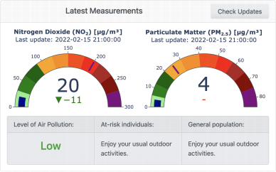
0-1. Gauges from Dashboard
Due to the high customization ability of the Plotly Graph Objects library, it was possible to design the gauges as planned. The dark blue shaded bar has a good contrast with the coloured arc, and the overall design is appealing and easy to interpret. The only minor weaknesses might be that the threshold line is not as outstanding as planned, but considering the background colours of its locations inside the two gauges, it was difficult to make it more apparent. The title and axis ticks are not distracting and fit well within the figure.
3.2 Historical data - Concentration vs Time
3.2.1 Questions the visualisation is intended to address
1. What were the concentrations of key air pollutants in the atmosphere in London Westminster at a certain time on a certain day?
2. How has the concentration of pollutants changed in over time in a certain period (quantitatively)?
3. Were the concentrations below the limit concentrations?
3.2.2 Target audience
![]() Scientific community, e.g., earth scientists, geoscientists, environmental scientists, and
Scientific community, e.g., earth scientists, geoscientists, environmental scientists, and
environmental engineers. They need access to reliable data to work on air pollution control and address these problems in detail. See Persona 1.
![]() Environmentalists, i.e., those concerned with and/or advocating for the protection of the
Environmentalists, i.e., those concerned with and/or advocating for the protection of the
environment. They may want to access the data and take some action depending on the current situation. See Persona 2.
![]() UK government bodies, such as Health and Safety Executive, Environment Agency and
UK government bodies, such as Health and Safety Executive, Environment Agency and
the Department for Environment, Food & Rural Affairs. They want to keep track of air pollutants levels to see the effects (or their absence) of the policies imposed by the Clean Air Strategy 2019 the progress towards the strict emission reduction targets. See Persona 3 .
![]() General public. One of the goals of the web application is to raise public awareness of air
General public. One of the goals of the web application is to raise public awareness of air
pollution, and this can be achieved by providing people with a solid evidence base, backed up by air quality data.
3.2.3 Data
For this visualization, the original dataset that includes hourly concentrations of air pollutants will be used, with no further data preparation necessary.
3.2.4 Chart type
Easy-to-read graphs of hourly data collected by OpenAQ, can allow to track changes in the air quality over time for audience of different technical expertise. Because the values of different air pollutants concentrations are typically very different in magnitude, it may be confusing to display them a single graph. For example, plotting concentration using two lines on a single line chart can be misleading as the concentration of NO2 is much higher PM2.5 concentration, and it will look like the PM2.5 concentrations are very small and not concerning, this can be very dangerous as the hourly mean NO2 concentration limit set by EU air quality standards is 200 μg/m3, while the limit daily concentration of PM2.5 is 25 μg/m3.
A great option to display a single line on the graph is an area chart. Area charts are like line charts but with the area underneath the line filled in with a certain colour or texture. They are particularly effective to show the evolution of quantitative values over time, and help to emphasize the overall trend, the peaks and troughs of the line that connects the data points. They are effective in that they communicate both the overall trend and at the same time showing the specific values.
Less technical audiences (e.g., general public, environmentalists) will be likely more interested in the overall trends, while more technical audiences (e.g., scientists, government authorities) will likely pick out some specific values. These charts are therefore very powerful, yet is easy to understand and interpret, and hence they will be useful for all audiences.
3.2.5 Design
Important parts of each chart include:
![]() A short title, that tells the quantity being shown, e.g., NO2 Concentration vs Time.
A short title, that tells the quantity being shown, e.g., NO2 Concentration vs Time. ![]() Axis with ticks representing the scale of possible values
Axis with ticks representing the scale of possible values
![]() Appropriate axis labels with units, e.g., Concentration (µg/m3)
Appropriate axis labels with units, e.g., Concentration (µg/m3)
![]() A limit concentration (based on WHO limits) drawn as a horizontal dashed line,
A limit concentration (based on WHO limits) drawn as a horizontal dashed line,
representing a threshold used to determine boundaries that visually alert the person looking at the chart if the concentrations are above this threshold.
![]() Grid lines, i.e., the lines that cross the chart plot to show axis divisions. They help
Grid lines, i.e., the lines that cross the chart plot to show axis divisions. They help
viewers of the chart see what value is represented by an unlabelled data point, thus helping to determine the actual values at a certain time.
3.2.6 Visual aspects
These charts do need to be very simplistic, yet the visuals and decorations should not be distracting. The lines and are fill should have similar shading, with the line being in darker that the filling, and the filling having a degree of transparency to allow viewers to see the grid behind it. The two charts need to have different colour pallets as to help the viewer distinguish between the two. Neutral colours should be used, such as blue and turquoise. Those are calm colours and are appealing for most people. Axis ticks must be small and light to avoid distraction. Labels need to match the style of the ticks but be a little larger and stand out a little more. Chart title needs to be readable but in light font and colour to avoid distraction. They will be in a similar style to axis labels but in a larger font size. The limit threshold concentration will be a red dashed line, so it stands out and is alerting. The grid must be visible but should not be distracting and interfering with the graph. Light grey lines will provide a way of linking line values to the axis but will not interfere with the plotted data line.
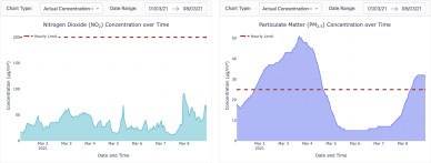
0-2. Concentration vs Time Area charts
It was possible to achieve the design described above. Since the area underneath the line is filled, the overall trends in pollutants concentrations are more apparent, and the figure does not seem so empty. The grid lines, axis ticks and labels, as well as the title are not distracting but are informative. The colour choices make the plotted line stand out from the rest of the figure and do look appealing. The limit red, dashed line is alerting and makes it easy to compare the concentration values to the health limit.
3.3 Historical data – Trends in Pollutant Levels over Time
3.3.1 Questions the visualisation is intended to address
1. How has the concentration of pollutants changed in over time in a certain period (qualitatively)?
2. Are the concentrations of pollutants increasing or decreasing since 2019?
3. Is there some hourly, daily, monthly, or annual trends in levels of key air pollutants?
3.3.2 Target audience
![]() Scientific community working to develop air pollution control measures and identify any
Scientific community working to develop air pollution control measures and identify any
important factors affecting it, that are not apparent at a first glance. See Persona 1.
![]() Environmentalists. They may want to assess the performance of the government in
Environmentalists. They may want to assess the performance of the government in
reducing air pollution and possibly do something depending on the situation. See Persona 2 .
![]() UK government bodies wanting to keep track of are pollution to see the effects strategies
UK government bodies wanting to keep track of are pollution to see the effects strategies
used in fighting it. See Persona 3.
![]() General public wanting to know how air quality is changing in time.
General public wanting to know how air quality is changing in time.
Hourly data on air pollutants levels is noisy, and as a result the graphs of actual concentration vs time can be difficult to read and pick up any trends. This could be because of high frequency random noise due to some error introduced in sensor measurement and signal transmission, or simply because air is moving due to wind etc., resulting in very quick movement of pollutants in the atmosphere.
If a person is not interested in the actual values but rather want to find the trends in the concentrations of the two pollutants, filtered data will be more convenient for it.
![]() The original prepared dataset will be used as the starting point but it requires some further
The original prepared dataset will be used as the starting point but it requires some further
![]() manipulation. A filtering algorithm can be used to remove noise from the data and the level of
manipulation. A filtering algorithm can be used to remove noise from the data and the level of
![]() filtering is determined by the filter’s frequency range and the filter removes data points that
filtering is determined by the filter’s frequency range and the filter removes data points that
![]() give rise to frequencies outside this range. In general getting rid of high frequencies gives more
give rise to frequencies outside this range. In general getting rid of high frequencies gives more
![]() smooth data curves that show how the pollutant levels vary with time. To do achieve this low pass filters e.g. a Butterworth lowpass filter can be used. By trial-and-error it was found that a Butterworth lowpass filter of order 3 with a critical frequency of 0.005 Hz gives the desired result. Critical frequency of 0.005 Hz means that the filter only keeps frequencies less than 0.005 Hz, resulting in a much smoother curve over long time periods, but it still shows enough detail as to accurately convey the overall trend in pollutants levels.
smooth data curves that show how the pollutant levels vary with time. To do achieve this low pass filters e.g. a Butterworth lowpass filter can be used. By trial-and-error it was found that a Butterworth lowpass filter of order 3 with a critical frequency of 0.005 Hz gives the desired result. Critical frequency of 0.005 Hz means that the filter only keeps frequencies less than 0.005 Hz, resulting in a much smoother curve over long time periods, but it still shows enough detail as to accurately convey the overall trend in pollutants levels.
3.3.4 Chart type
Again to avoid viewer confusion its best to use separate graphs for different pollutants.
Similar considerations apply to these graphs as for historical graphs, and hence an area chart will be used.
3.3.5 Design
![]() This time however the graphs will only be used to show trends rather than convey specific values and hence any y-axis labels will be omitted since they have no real meaning and may mislead the viewers.
This time however the graphs will only be used to show trends rather than convey specific values and hence any y-axis labels will be omitted since they have no real meaning and may mislead the viewers.
Important parts of each chart include:
![]() A short title, that tells what is being shown, e.g., NO2 Time Trend
A short title, that tells what is being shown, e.g., NO2 Time Trend
![]() X-Axis with ticks the time scale.
X-Axis with ticks the time scale.
![]() Grid lines. Although they have no real meaning for the y-axis, the grid still helps the
Grid lines. Although they have no real meaning for the y-axis, the grid still helps the
viewers to compare the levels of pollutants between different time points.
3.3.6 Visual aspects
Similar considerations regarding the visual aspects apply as for the concentration-time graphs. (See Visualisation 2). In fact, the charts will be created simply by switching the data used to plot the graphs, as well as modifying the title and the y-axis. On the dashboard, it will be
![]() convenient to allow the user to change the chart type from actual concentration to the
convenient to allow the user to change the chart type from actual concentration to the
![]() trendline chart within a single dashboard element. Therefore the visual aspects of the design
trendline chart within a single dashboard element. Therefore the visual aspects of the design
![]() will stay the same as to keep the visualization look the same while showing different
will stay the same as to keep the visualization look the same while showing different
information.
3.4 Air quality distribution in a time period
3.4.1 Questions the visualisation is intended to address
1. How is the air pollution distributed over some time period (e.g., last week, part 365 days, 19/01/19 – 16/04/21)?
2. How many days was the air quality falling under a certain band over some time period?
3. How was the general air quality in some time period?
3.4.2 Target audience
![]() Environmentalists. They may want to know the overall level of air pollution and although
Environmentalists. They may want to know the overall level of air pollution and although
it might be decreasing, it may still be bad, and they will want to do soothing about it. See Persona 2.
![]() Relevant UK government bodies want to know what the overall level of air pollution in
Relevant UK government bodies want to know what the overall level of air pollution in
the area is, and whether they need to implement new strategies or more strict policies to fight it. See Persona 3.
![]() At-risk individuals (e.g., elderly or people with heart problems), or parents of young
At-risk individuals (e.g., elderly or people with heart problems), or parents of young
children considering moving into the area. They might want to know the general level of air quality and decide whether they want to move to live in the area or not.
![]() General public wanting to know how what the air quality in the area is.
General public wanting to know how what the air quality in the area is.
3.4.3 Data
For this visualization, the newly prepared categorical datasets will be used, that link the days to the air pollution bends based on concentration of each pollutant as well as global that considersth both.
3.4.4 Chart type
This visualisation consists not only of one chart, but of three charts, representing the air quality levels based on NO2 concentration, PM2.5 concentration and global index (taking into account both pollutants). In all cases the highest hourly Index level (i.e., the worst air quality category) in a day determines the daily Index level taken into account.
To show the proportions and percentages between air quality categories, a donut chart will be used. They are effective in showing proportional distribution of ordinal (categorical) data, especially when the number of categories is small. A donut chart like a pie chart but with an area of the centre cut out. Each arc length represents a proportion of each category, while the full circle, or donut represents the total sum of all the data, equal to 100%. Pie charts are often criticised confusing the viewer and focusing them on the proportional areas of the slices to one another and to the chart as a whole, making it difficult to see the differences between slices. A donut chart, on the other hand, de-emphasizes the use of the area, and brings the viewers focus to comparing the length of the arcs, rather than comparing the proportions between slices. They are also more space-efficient, and the blank space inside the donut can be used to display information inside it.
3.4.5 Design
Important parts of each chart include:
A short title inside the donut, that tells what is being shown, e.g., NO2 . Annotations inside each arc with the relative value (percentage) of each arc, i.e., the percentage of days falling under this category.
Legend, linking the colour of each arc to the air pollution bend it represents.
3.4.6 Visual aspects
All charts should be well-formatted, and no 3D elements or exploding slices will be used as these are confusing. The size of the hole will be half of that of the overall circle. The chosen colour pallet for the arcs includes green (Low pollution level), orange (moderate pollution levels), red (high pollution level) and purple (very high pollution level), as these are intuitive for most people.
The annotations will be in dark colour and in light font, positioned inside the arc if size allows, or outside if the arc is too small. The title will be in dark colour that gives a contrast with the donut itself, and will be positioned in the middle of the donuts hole and sized to fit appropriately allowing for a small margin between the text and the arcs. The legend will be on the left of the donut, and if positioned side-by-side may serve as one for multiple donuts.
3.4.7 Design Evaluation
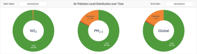
The final result achieved in a bit different to the design described above. First, it was found difficult to position a legend for the donuts such as to keep the size of all the donuts the same. It was attempted to have the legend only for the last donut chart, as they are placed side by side and the legend stays the same. Nevertheless, the size of the last donut was always smaller, and it would not look appealing. The legend did take up too much space as well. It was therefore decided to not have the legend, and use annotations inside each arc to note the air pollution bend the arc represents. It was also found that in case some ark becomes too small for the annotations to fit inside and still be readable, the outside annotation changes the size of this donut. As to keep the size of all the donuts the same, and keep the overall style of the chart appealing, it was decided to omit any annotations in case they do not fit. This is convenient since the pollution level each arc represents is indicated in the hover when hovering over the donut (as part of Plotly functionality), so that the viewer may easily identify what this arc represents. Not to mention that since the colour map used to match colours and pollution bands they represents is kept the same in all visualizations, it will likely be intuitive for the viewer to understand straight away what ark is what without even hovering over it. Otherwise, the final design matches all the criteria set above.
3.5 Daily air quality distribution
3.5.1 Questions the visualisation is intended to address
1. How is the pollution level distributed throughout the day by hours?
2. When is the air quality expected to be best or worst throughout the day?
3. When is the best time of the day to do outdoor activities?
3.5.2 Target audience
![]() At-risk individuals living in the area, e.g., people with lung or heart problems, people with
At-risk individuals living in the area, e.g., people with lung or heart problems, people with
asthma and elderly.
![]() Athletes, such as people who want to go for a run outside, exercise in a park, or some
Athletes, such as people who want to go for a run outside, exercise in a park, or some
other sort of outdoor training.
![]() Parents of young children.
Parents of young children.
![]() Pregnant women.
Pregnant women.
![]() Outdoor workers and their employers.
Outdoor workers and their employers.
All the aforementioned groups of people will find it useful to know the distribution of air quality throughout the day and use it to make prediction of the air quality at a certain time of the day.
Knowing the current air quality is good, but people generally want to plan their day in advance and to aid their planning they will want to know when to schedule their outdoor activities such that the air quality at that time will likely be good. On the other hand, if it is impossible to plan the days such that the outdoor activities are carried out at the time when air quality is best, it is useful to know when it is likely to be worst, and exclude these time from the list of possible choices.
The sample size of the data is large, and therefore statistically meaningful and thus can be used to make predictions. It is expected that there are some daily air quality trends, for instance it is likely that the air quality in the evening, when most people are already home and there are less cars on the roads, is going to be better than in the morning when people are rushing to work. Now the aim of this visualization is to help identify those trends and communicate them to the
2023-02-07