Hello, dear friend, you can consult us at any time if you have any questions, add WeChat: daixieit

Problem 1 (50 points, Bayesfilter). In this problem, we are given a robot operating in a 2D grid world. Every cell in the grid world is characterized by a color (0 or 1). The robot is equipped with a noisy odometer and a noisy color sensor. Given a stream of actions and corresponding observations, implement a Bayes filter to keep track of the robot’s current position. The sensor reads the color of the cell of the grid world correctly with probability 0.9 and incorrectly with probability 0.1. At each step, the robot can take an action to move in 4 directions (north, east, south, west). Execution of these actions is noisy, so after the robot performs this action, it actually makes the move with probability 0.9 and stays at the same spot without moving with probability 0.1.

When the robot is at the edge of the grid world and is tasked with executing an action that would take it outside the boundaries of the grid world, the robot remains in the same state with probability 1. Start with a uniform prior on all states. For example if you have a world with 4 states (x1,x2,x3,x4) then P(X0 = x1) = P(X0 = x2) = P(X0 = x3) = P(X0 = x4) = 0.25.

You are given a zip file with some starter code for this problem: this consists of the Python scripts example_test.py and histogram_filter.py (Bayes filter is also called the Histogram filter) and a starter file containing some data: starter.npz. The starter.npz file contains a binary color-map (the grid), a sequence of actions, a sequence of observations, and a sequence of the correct beliefstates. Thisis provided for you to debug your code. You should implement your code in the histogram_filter.py. Be careful not to change the function signature, or your code will not pass the tests on the autograder. You will turn in your assignment using Gradescope.

Problem 2 (35 points, Learning HMMs). In this problem, we are going to implement what is called the Baum-Welch algorithm for HMMs. Recall that an HMM with observation matrix M has an underlying Markov chain with an initial distribution π and state-transition matrix T . Let us denote our HMM by

λ = (π,T,M ).

Say someone had given us an HMM λ which gave us a sequence of observations Y1,...,Yt. Since these observations happened, they tell us something more about our given state- transition and observation matrices, for example, given these observations, we can go back and modify T,M to be such that the observation sequence is more likely, i.e., it improves

Y1,...,Yt | λ).

(a) (20 points) Assume that we are tracking a criminal who shuttles merchandise between

P

(

Los Angeles (x1) and New York (x2). The state transition matrix between these states is

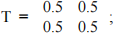
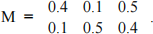
e.g., given the person is in LA, he is likely to stay in LA or go to NY with equal probability. We can make observations about this person, we either observe him to be in LA (y1), NY (y2), or do not observe anything at all (null, y3).

Say that we are tracking the person and we observed an observation sequence of 20 periods (null, LA, LA, null, NY, null, NY, NY, NY, null, NY, NY, NY, NY, NY, null, null, LA, LA, NY). Assume that we do not know where the criminal is at the first time-step, so the initial distribution π is uniform.

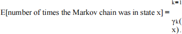
We first compute the probability of each state given all the observations, i.e.,

γk(x) = P(Xk = x | Y1,...,Yt,λ) = αk(xx)αβt(kx(x) ) .

which is simply our smoothing probability computed using the HMM λ computed using the rd and backward variables αk ,βk . You should check that γk (x) should be a legitimate probability distribution, i.e., x γk(x) = 1.

Compute the smoothing probabilities γk (x) for all 20 time-steps and both states and show it in a table like we had in the lecture notes. You should also show the corresponding tables for the forward and backward probabilities αk s and βk s.

You should get the point-wise most likely sequence of states after doing so to be (LA, LA, LA, LA, NY, LA, NY, NY, NY, LA, NY, NY, NY, NY, NY, LA, LA, LA, LA, NY). Notice how smoothing fills in the missing observations above.

(b) (5 points) We now discuss how to update the model λ given our observations. First observe that

Let us define a new quantity

ξ k(x,x′) = P(X k = x,Xk+1 = x′ | Y 1 ,...,Yt,λ )

to be the probability of being at a state x at time k and then moving to state x′ at time k + 1, conditional upon all the observations we have received from our HMM. Show that

ξk(x,x′) = η αk(x)Tx,x′ M x′,yk+1 βk+1(x′)

where η is a normalizing constant that makes x,x′ ξk(x,x′) = 1.

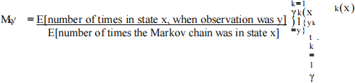
(c) (5 points) We can now use our estimate from the previous part to get

We now construct an updated model for our HMM asfollows. The initial distribution of the states, instead of being π, is our smoothing probability

π′ = γ1(x).

Entries of the new transition matrix can be computed by

Entries of the new observation matrix can be computed by

= (π′,T ′,M ′)

Write down the new HMM model λ′ and see if any entires have changed as compared to λ.

λ

′

(d) (5 points) Compare the two HMMs λ and λ′. Compute the two probabilities and show that

...,Yt | λ) < P(Y1,...,Yt | λ′).

This is exactly what Baum et al. proved in the paper Baum, Leonard E., et al. "A

P(

Y 1,

maximization technique occurring in the statistical analysis of probabilistic functions of Markov chains." The annals of mathematical statistics 41.1 (1970): 164-171. You can see that the Baum-Welch algorithm is quite powerful to learn real-world Markov chains, e.g., the running gait of your dog (what is the state here?) given observations of its limb positions. Given some elementary model of the dynamics T and an observation model M , you can sequentially update both of them to guess a better model of the dynamics.