ECMT6006 2021S1 Assignment 2

Due: 23:59 Sunday 6 June 2021

        Please compile your solutions in ONE file (not including the program code which you can submit separately) and submit it via Turnitin in Canvas. You can either handwrite or type your answers. For the empirical questions, please present the figures and provide your analyses/interpretations properly. If you use MATLAB, you can present your answers using livescript exported in a doc-ument format. Except for special circumstances, I DO NOT accept late sub-mission.

        Note: Patton (2019) refers to the reference textbook by Andrew Patton.

Question 1. Question 3 in Section 5.10.2 on Page 185 in Patton (2019).

Question 2. Question 4 in Section 5.10.2 on Page 186 in Patton (2019).

Question 3. In this question, you will use the S&P500 index daily prices¹ over the period 2010–2015. Please convert the daily prices into continuously compounded returns, and then use the return series to answer the following questions.

(i) Consider a ARMA(p, q) conditional mean model (allowing for the constant term) for the returns with p = 0, 1, . . . , 5 and q = 0, 1, . . . , 5. Use the three information criteria discussed in class (AIC, HQIC, BIC) to select the best model. Report your results.

(ii) Obtain the residuals from the conditional mean model selected by BIC, and estimate a GARCH(1,1) model using the residuals. Report the estimated parameters in this conditional mean and conditional variance model

(iii) Plot the estimated conditional volatility in annualized standard deviation².

Question 4. Use the 2010–2015 daily S&P 500 index returns that you obtained for Question 3, estimate the conditional 5%-VaR using the below two methods.

(i) (Historical Simulation) Use the daily data in the whole year 2010 to ob-tain the empirical distribution of the return on the first day of 2011, and compute the 5%-VaR on the first day of 2011. Next, repeat this day after day using a one-year rolling window, and obtain the daily VaR forecast from 2011 to 2015.

(ii) (Parametric GARCH Model) Assume the daily returns follow the below model with constant conditional mean and GARCH(1,1) conditional vari-ance:

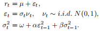
Estimate the daily conditional 5%-VaR process and and make a time-series plot of it.

Question 5. Question 1 in Section 9.10.2 on Page 331 in Patton (2019).

Question 6. Question 2 in Section 9.10.2 on Page 333 in Patton (2019).

Question 7. (Forecasting evaluation and comparison) You can find monthly term premium on a 10-year zero coupon bond from April 1953 to December 2013 (T = 729 observationss) in the file “term premium.xlsx”. In this exercise, you will use this dataset to (a) generate forecasts using an ARMA(1,1) and a “Random Walk” model, (b) evaluate the optimality of the model forecasts, and (c) compare these two model forecasts.

(i) Generate a time-series plot of the term premium data in the data file term premium.xlsx, with a proper x-label and y-label.

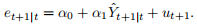
(ii) Use the first half of the sample (first R = 364 observations from April 1953 to July 1983) to estimate a stationary ARMA(1,1) model

and obtain the parameter estimates .

(iii) What is the feasible one-step-ahead forecast ?

(iv) Let ,³ compute  for t = 0, 1, . . . , T − 1 and plot them together with the real data Yt for t = 1, . . . , T. 

(v) Note that for t = R, . . . , T −1 are fixed window forecasts in the out-of-sample analysis of the above ARMA(1,1) model. Compute the forecast errors , and generate a time series plot of them.

(vi) What would you expect for the serial correlation of the forecast errors if the above forecasts are optimal? Plot the sample ACF of the forecast error series {, t = R, . . . , T −1}, and conduct bot Ljung-Box test and robust test on the joint serial correlation with lages L = 5, 10, 20. What is your conclusion by examining the ACF plot and the test results?

(vii) The “Mincer-Zarnowitz” (MZ) regression⁴ regresses the realized data on its forecast and a constant. The null hypothesis is that the intercept is 0 and the slope is 1. Now consider an alternative and equivalent formulation: 

What parameter restrictions would you test in this regression to examine the optimality of ? Run regression (1) using your data on and  for t = R, . . . , T − 1, and conduct a test to draw conclusion on the optimality of your forecasts.

(viii) Now consider an alternative model

which is a “Random Walk”. What is the best one-step-ahead forecast Yˆt+1|t for this model?

(ix) Repeat steps (v), (vi), (vii) for the Random Walk model.

(x) Compare the forecasts from the ARMA(1,1) model and Random Walk model by a “Diebold-Mariano” (DM)⁵ test with a squared error loss func-tion. Specifically, the difference of the two losses is

where denote the forecast errors from the ARMA(1,1) model and Random Walk model respectively. Conduct a DM test by testing the zero mean of dt using a robust t-test with both White and Newey-West robust errors. Draw your conclusion on which model is better in terms of forecasting power.

Question 8. Question 1 in Section 11.7.2 on Page 408 in Patton (2019)

Question 9. Question 2 in Section 11.7.2 on Page 409 in Patton (2019)