STAT 151 LAB 1 ASSIGNMENT
Hello, dear friend, you can consult us at any time if you have any questions, add WeChat: daixieit
LAB 1 ASSIGNMENT
Due Date: February 3 at 9:59 PM
DISPLAYING AND DESCRIBING DISTRIBUTIONS
IMPORTANT:
1) In this lab, you will need to use graphical and numerical tools in R or (R commander) to generate the outputs.
2) For all graphs and charts, please label the axes and ensure proper titles are used.
3) For all tables, please ensure the correct variable name(s) are used.
4) Each group will be expected to create a Google document for the lab report where students will type their answers (in full sentences) and paste the R output (where necessary) for each lab question.
5) Completed assignments will be saved as a PDF file, submitted, graded, and returned on eClass.
6) Each lab group MUST upload and submit only ONE lab report, so students MUST work on EVERY question together to complete the lab assignment together. In other words, students are NOT allowed to divide the lab and do a portion of the lab.
7) Please see the Lab Submission Info tab through the Lab Information link in the Labs section on eClass.
In this lab assignment, you will use graphical and numerical tools in R to explore the data about greenhouse gas (GHG) emissions reported from more than one hundred Alberta facilities in a 13-year period (2004-2016). You will examine the distribution of GHG emissions in 2016 as well as analyse the trend and changes in the distribution of GHG emissions over the aforementioned period. You will also identify the largest emitters and compare Alberta industrial sectors in terms of their total GHG emissions. In particular, you will assess the impact of Oil Sands on GHG emissions. The questions in the lab assignment refer to the R tools discussed in the Lab 1 Instructions.
Alberta Facility Greenhouse Gas Emissions
Global warming is driven mainly by the following greenhouse gases (GHG): carbon dioxide (CO2), methane (CH4), nitrous oxide (N2O), hydrofluorocarbons (HFC), perfluorocarbons (PFC), and sulphur hexafluoride (SF6). GHGs are not equal in their effect on the atmosphere, however; each GHG has a unique average atmospheric lifetime and heat-trapping potential. GHG emissions are often calculated and reported in terms of how much CO2 would be required to produce a similar warming effect over a given time horizon (usually 100 years). This is called the CO2 equivalent (CO2e) value and is calculated by multiplying the amount of the gas by its associated global warming potential. The idea is to express the impact of each different greenhouse gas in terms of the amount of CO2 that would create the same amount of warming.
Since 2004, the Government of Alberta has required industrial facilities across the province to report their GHG emissions annually through the Alberta Specified Gas Reporting Regulation program. Initially, the program had applied to all facilities that emit the equivalent of 100,000 tonnes (100 kilotonnes, or 100 kt) or more of GHGs in CO2 per year. This threshold was lowered to 50 kt for the 2010 calendar year and subsequent reporting years. Note that the program just covers industrial sources; emissions from other sources including transportation, agriculture, commercial, and residential are not included in the inventory. According to a 2013 report, reported industrial emissions accounted for 49.7% of Alberta’s total emissions.
In this lab assignment, you will examine the greenhouse gas data from up to 280 facilities in Alberta in a 13-year period (2004-2016). The data are posted under Open Government License- Alberta at https://open.alberta.ca/dataset/specified-gas-reporting-regulation-summary.
This dataset is available in the Data link located in the Lab 1 tab display in the Labs section on eClass. Please import the data into R. (Hint: Students should use “Tabs” as “Field Separator” to import the data set into R Commander.) The data are not to be printed in your submission. The following is a description of the variables in the data file:
Variable Name Description of Variable
YEAR Year in which the values of the emissions were obtained,
SECTOR Industry type,
LEGAL.NAME Legal name of a corporation.
FACILITY Facility Name,
TOTAL Total CO2 equivalent emissions (in tonnes).
NOTE: You might need to write some R commands to obtain some outputs. Therefore, reading R instruction files available on eClass is recommended.
1. Before carrying out statistical analysis, examine the study design.
(a) Is this an observational study or an experiment? Can the results of the study be extended to the population of interest which is all GHG emitting facilities worldwide? Are causal inferences possible?
(b) In the 2004 – 2009 period, the mandatory threshold for reporting emissions was 100 kt. This threshold was lowered to 50 kt for the 2010 calendar year and subsequent reporting years. Obtain the frequency table of the number of facilities by year. How may this change affect any comparisons in total emissions for years before and after the threshold change?
2. Now examine the reported Alberta greenhouse gas emissions for 2016.
(a) Obtain the summary statistics (mean, standard deviation, IQR, min, Q1, median, Q3, max, and n) for TOTAL in 2016. Report the summary statistics and answer these questions: How many facilities reported emissions in 2016 and what was the sum of all their total CO2e emissions? What are the corresponding mean, standard deviation, and maximum value? What are the three quartiles? Compare the mean with the median. Is the expected distribution shape of TOTAL symmetric, right-skewed, or left-skewed? (Consider reporting values in megatons (Mt), where 1 Mt = 1 million tonnes or 1,000 kilotons, for better clarity.)
(b) How many facilities reported their emissions voluntarily in 2016? Using all facilities listed, what is the percentage of facilities that reported their emissions voluntarily in 2016? What is the percentage contribution to TOTAL for these facilities in 2016?
(c) Which facility in Alberta had the largest value for TOTAL in 2016? What was the value in that year? What was the percentage contribution of this value from the single facility to the sum of TOTAL? Compare the contribution to the percentage contribution in part (b).
(d) What is the 95th percentile of TOTAL and what is the percentage contribution to TOTAL of the remaining 5% of the facilities? Report the appropriate values from the output. There is no need to paste the outputs into your report.
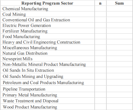
(e) What were the sums of TOTAL for each of the 18 sectors in 2016? In that year, which sector reported the largest share of total CO2e emissions in Alberta and what was its percentage contribution? You do not need to paste the output in your report. Simply copy the following table to your report and fill it out. Also, obtain a pie chart to display the contribution of each sector for TOTAL in 2016. Paste the chart into your report. Comment briefly on the largest and smallest sectors.
(f) Obtain a frequency histogram of TOTAL in 2016 with bins starting at 0 and a width of 1,000,000. (Hint: R assumes that the right endpoint of each interval is included. Your histogram should include the left endpoints.) Paste the plot into your report. The histogram should have proper title and axis labels. Describe the shape of the histogram. What do you conclude about the distribution of TOTAL in 2016?
3. Now explore long-term trends in reported GHG emissions in Alberta. In order to meaningfully compare the data over time, emissions from facilities reporting their emissions voluntarily must be excluded. Therefore, for the comparisons over the entire period (2004 – 2016), consider only facilities whose emissions are 100 kt CO2e or more.
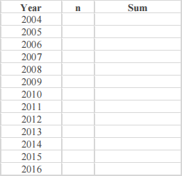
(a) For each year of the period (2004 - 2016), obtain the sum of TOTAL for all facilities with TOTAL at 100 kt or more. You do not need to paste the summaries into your report. Simply copy the following table to your report, fill it out and, based on the summaries, calculate the percentage increase in total emissions over the entire period. (Hint: You may use the tapply() function to find the sum of TOTAL.)
(b) Obtain a timeplot for the summaries obtained in part (a). Paste the plot into your report. Comment about the change in TOTAL over the period.
(c) Obtain side-by-side boxplots of TOTAL by Year for all facilities with TOTAL at 100 kt or more for each year of the period (2004 – 2016). Click “Options” and select “With mouse” when you make the boxplot in R commander to see which observations identify as outliers. Paste the graph into your report. Compare the centers, spreads, and shapes of the 13 distributions and provide a brief summary. Identify the facilities that are the largest emitters over the period (hover the cursor over the outliers). If the same facility appears more than once as the largest emitter in the period, assess progress in reducing emissions in the facility over time. (Note that some facilities may have slightly different names from year to year.)
(d) Comment on what information about emissions derived from the timeplot in part (b) and the side-by-side boxplots in (c) can be observed. What information can be derived from one plot but not from the other? Explain briefly.
4. In this question, assess the impact of the Oil Sands industry on TOTAL in the period (2004 – 2016).
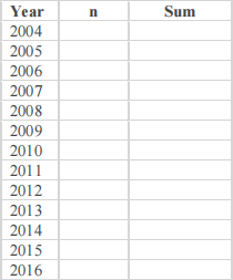
(a) Obtain the summary statistics (mean, standard deviation, IQR, median, and number of facilities) for TOTAL for the combined “Oil Sands In Situ Extraction” and “Oil Sands Mining and Upgrading” sectors. For each year in the period (2004 - 2016), include only facilities with TOTAL at 100 kt or more. Paste the output into your report. Then find sums, copy the following table to your report, and fill it out. (Hint: You may use the tapply() function to find the sum of TOTAL.)
Comment on the change in the number of facilities from 2004 to 2016 and the change in total emissions from the Oil Sands in this time period. Also, comment on how the summary statistics changed for the total emissions by this industry in the period. In particular, compare the mean with the median, comment about the skewness of the distribution, and which measures of center and spread should be used.
(b) Obtain a timeplot for the sums obtained in part (a). Paste the plot into your report. Comment about the change in TOTAL in the Oil Sands sectors over the period.
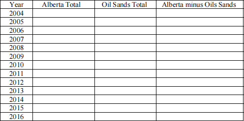
(c) Obtain a new variable “Alberta minus Oils Sands”, which is the difference of “Alberta TOTAL for all facilities with TOTAL at 100 kt or more” (the sums obtained in Question 3a) and the emissions of the combined Oil Sands categories (the sums obtained in Question 4a). Copy the following table of summaries to your report and fill it out.
Comment about the change in TOTAL for Oil Sands facilities and the change in TOTAL for all Alberta facilities without Oil Sands facilities in the period (2004 – 2016) (specifically, compute the percentage change from 2004 to 2016 in each case). Then use the summaries to obtain a timeplot with two lines over the period: 1) TOTAL for all Alberta facilities without Oil Sands facilities and 2) Oil Sands emissions only. Paste the chart into your report. Comment briefly.
LAB 1 ASSIGNMENT: MARKING SCHEMA
Proper cover page (use "Lab Assignment Template" on eClass for proper format) and appearance (lab reports must be typed): 10 marks
Question 1 (8)
(a) Observational study or experiment: 2 marks
Population Inferences: 1 mark
Causal Inferences: 1 mark
(b) Table of number of facilities: 2 marks
Effect of change in the threshold value: 2 marks
Question 2 (50)
(a) R output for Summary Statistics: 2 marks
Total number of facilities: 2 marks
Sum of TOTAL: 2 marks
Mean, standard deviation, and max values: 3 marks (1 each)
Quartiles: 3 marks (1 each)
Comparison of mean and median, expected shape of distribution: 4 marks (2 each)
(b) Number and percentage of voluntary facilities in 2016: 2 marks
Percentage contribution to TOTAL: 2 marks
(c) Largest emitter and value in 2016: 2 marks
Comparison with value from part (b): 2 marks
(d) 95th percentile: 2 marks
Percentage contribution to TOTAL of top 5%: 2 marks
(e) Sums of TOTAL for each of the 18 sectors in 2016: 4 marks
Sector with the largest TOTAL sum in 2016: 2 marks
Percentage contribution of the sector: 2 marks
Pie chart for TOTAL sums for 18 sectors: 4 marks
Comments: 2 marks
(f) Properly formatted frequency histogram of TOTAL in 2016: 4 marks
Shape: 2 marks
Conclusions: 2 marks
Question 3 (28)
(a) Sum of TOTAL for all facilities with TOTAL at 100 kt or more for each year: 2 marks
Percentage increase in TOTAL: 2 marks
(b) Timeplot: 4 marks
Comments: 2 marks
(c) Side-by-side boxplot (with proper format) of TOTAL by Year: 4 marks
Summary comments about the centers, spreads, and shapes of the 13 distributions: 4 marks
Largest emitter(s): 2 marks
Progress in reducing emissions by the largest emitter(s) over the period: 2 marks
(d) Comparison: 3 marks
Information derived from one plot but not the other: 3 marks
Question 4 (33)
(a) Summary statistics: 5 marks
Fill in the table: 2 marks
Comments about change in total emissions for Oil Sands: 2 marks
Compare mean and median: 1 mark
Shape of the distribution: 1 mark
Measure of center: 1 mark
Measure of spread: 1 mark
(b) Timeplot: 4 marks
Comments: 2 marks
(c) Summaries: 4 marks
Comments using percentage changes: 3 marks
Timeplot: 4 marks
Timeplot interpretation: 3 marks
TOTAL = 129
2023-02-03