MAST20004 Probability Semester 1, 2021
Hello, dear friend, you can consult us at any time if you have any questions, add WeChat: daixieit
MAST20004 Probability
Semester 1, 2021
Question 1 (7 marks)
Events A and B satisfy P(A) = ![]() , P(A \ B) =
, P(A \ B) = ![]() and P(Ac \ B) =
and P(Ac \ B) = ![]() .
.
(a) Compute
(i) P(Ac ).
(ii) P(B|A).
(iii) P(B).
(iv) P(Ac |Bc ).
(b) Is there a positive or negative relationship between the two events A and B? Explain.
Question 2 (9 marks)
A student takes a multiple choice exam in which each question has 5 choices, exactly one of which is correct. If the student knows the correct answer, then they select that answer. Otherwise, they select an answer equally likely from the 5 choices. Suppose the student knows the answer to 50% of the questions.
(a) What is the probability that the student gets a correct answer to a given question?
(b) If the student gets the correct answer to a given question, what is the probability they knew the correct answer?
(c) For an exam with 20 questions, state the assumption(s) and derive the probability that they get correct answers to at least 12 questions. (No need to compute the final numerical answer.)
Question 3 (10 marks)
Let A,B,C be three events with P(A) > 0, P(B) > 0 and P(C) > 0. For each of the following statements, determine whether it is true or false. If it is true, give a proof; if it is false, give a counterexample.
(a) If P(A [ B) = P(A)+ P(B), then A \ B = ;.
(b) If P(A|B \ C) = P(A|B), then P(A \ C|B) = P(A|B)P(C|B).
(c) Assume that A, B and C satisfy two assumptions: (i) A and B are mutually independent, (ii) A and C are mutually independent; then A and B \ C are mutually independent.
(d) If f and g are two probability density functions, then ![]() (f + g) is also a probability density function.
(f + g) is also a probability density function.
(e) For a continuous nonnegative random variable X, if E(X2) exists, then E(X) exists.
Question 4 (10 marks)
A continuous random variable X has probability density function given by
fX (x) = ![]()
where c is a constant.
(a) Find the value of c.
(b) Find the cumulative distribution function FX of X .
(c) Find the mean and variance of X .
(d) Use the Bienaym´e-Chebyshev inequality to give a lower bound for the probability that X takes values within 3 standard deviations of its mean and compare it with the actual probability. Comment on your findings.
(e) Let Y = log(X2). Find the probability density function of Y .
Question 5 (15 marks)
Accidents in a Poisson town happen according to a Poisson process with rate one accident per week, and the cost of the damage caused by each accident is an exponential random variable with mean $1000, independent of other accidents.
(a) Find the probability that in a given week there are at least 2 accidents.
(b) An accident with a cost of damage less than $500 is classified as a minor accident. For a week with X accidents in the Poisson town, let M be the number of minor accidents in that week.
(i) Compute the conditional probability mass function of M given X = n for n = 0, 1, 2, . . . .
(ii) Derive the probability mass function of M .
(c) Let T be the total cost of damage in a week caused by the accidents in the Poisson town.
(i) Represent T as a suitable sum and state the assumptions.
(ii) Compute E(T|X) and Var(T|X).
(iii) Compute the mean and variance of T using the formulas E(T) = E{E(T|X)} and
Var(T) = E{Var(T|X)} + Var{E(T|X)}.
(iv) Four students wrote Matlab programs for simulating the values of E(T) and Var(T), only one of them is correct. Which of them is correct?
(I)
nreps=10000 ;
for i=1:nreps
N=randpois(1,1);
T(i)=sum(-log(1-rand(N,1))/1000);
end
Tmean=mean(T)
VarT=std(T)^2
(II)
nreps=10000 ;
for i=1:nreps
N=randpois(1,1);
T(i)=sum(-(1-randn(N,1))/1000);
end
Tmean=mean(T)
VarT=std(T)^2
(III)
nreps=10000 ;
for i=1:nreps
N=randpois(1,1);
T(i)=sum(-1000*(1-randn(N,1)));
end
Tmean=mean(T)
VarT=std(T)^2
(IV)
nreps=10000 ;
for i=1:nreps
N=randpois(1,1);
T(i)=sum(-1000*log(1-rand(N,1)));
end
Tmean=mean(T)
VarT=std(T)^2
Question 6 (13 marks)
The joint probability density function of the random variables X and Y is given by
f(x,y) = ![]()
(a) Draw the support of (X,Y).
(b) Show that c = ![]() .
.
(c) Determine the marginal probability density function of X .
(d) Determine the conditional probability density function of Y given X = x.
(e) Are X and Y independent? Explain.
(f) Compute the probability P(Y > 1|X = ![]() ).
).
(g) Compute the probability P(Y > 1).
Question 7 (10 marks)
Let P be a random point uniformly distributed inside the unit circle, and let (X,Y) be the Cartesian coordinates of P. The joint probability density function of (X,Y) is thus given by
|
8 1 f(X,Y )(x,y) = < ⇡ , : 0, |
0 < x2 + y2 < 1, elsewhere. |
(a) Derive the joint and marginal probability density functions for the polar coordinates
(R,⇥) of P. Check that your marginal probability density functions integrate to 1 over the appropriate domain.
(b) Are the polar coordinates independent?
(c) Derive the cumulative distribution function FR for R.
(d) Explain how you would use FR to generate an observation of R from an observation of U ![]() R(0, 1).
R(0, 1).
(e) Explain how to modify the joint probability density functions f(X,Y )(x,y) and f(R,⇥)(r,✓) in order for P to be a random point uniformly distributed inside the first quarter of the unit circle:
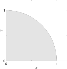
Does that modify the marginal distributions of the polar coordinates R and ⇥? Give a simple argument without computation.
Question 8 (6 marks)
Let (X,Y) be a general bivariate normal random variable.
(a) If Cov(X,Y) = 0, show that X,Y are independent.
(b) If Var(X) = Var(Y), show that Cov(X + Y,X − Y) = 0.
(c) Assume that µX = 0, σX(2) = 1, µY = −1, σY(2) = 4, and p = 1/2. We can show that X +Y is a normal random variable with mean µX+Y = E(X +Y) and variance σX(2)+Y = Var(X + Y).
Compute µX+Y and σX(2)+Y, and then write an expression for P(X + Y > 0) in terms of the cumulative distribution function of the standard normal distribution. No numerical answer is required.
Question 9 (15 marks)
Let X be a geometric random variable with parameter (success probability) p = 3/4, and let X1,X2 , . . . ,Xn be independent and identically distributed copies of X . Let Sn = X1 + X2 + ··· + Xn .
(a) Prove that the mgf (moment generating function) of X is MX(t) = ![]() , and determine the domain of values of t for which it is well defined.
, and determine the domain of values of t for which it is well defined.
(b) Find the mgf MSn(t) of Sn . Then state the distribution of Sn .
(c) Find the mgf M![]() n (t) of the sample mean
n (t) of the sample mean ![]() n =
n = ![]() .
.
(d) Find the limit limn!1 M![]() n (t) using the result of (c). What distribution does the limiting mgf correspond to? Interpret your result.
n (t) using the result of (c). What distribution does the limiting mgf correspond to? Interpret your result.
(e) Let
![]() Zn =
Zn = ![]() ^n ✓
^n ✓![]() n −
n − ![]() ◆ .
◆ .
Find MZn(t), the mgf of Zn . Then find the limiting mgf limn!1 MZn(t). What is the limiting distribution of Zn? Interpret your result.
Question 10 (10 marks)
Suppose brands A and B have consumer loyalties of 0.7 and 0.8, meaning that a customer who buys A one week will with probability 0.7 buy it again the next week, or try the other brand with probability 0.3. Let Xn be the brand bought by a specific customer on Week n, n ≥ 1.
(a) Model {Xn} as a Markov chain by determining the state space S and the transition matrix P .
(b) If Peter buys brand A on Week 1, what is the probability that he is loyal and keeps buying brand A for the next two weeks?
(c) If Peter buys brand A on Week 1, what is the probability that he buys brand A on Week 3? Note that this is a di↵erent question from (b).
(d) What is the limiting market share for each of these brands?
(e) Suppose now that there is a third brand with loyalty 0.9, that the third brand does not influence the loyalties of the first two, and that a consumer who changes any brand picks one of the other two with equal probability. If Xn still denotes the brand bought by a specific customer on Week n (n ≥ 1), what is the new state space S, and transition matrix P corresponding to the Markov chain?
(f) What conclusion can be drawn from the following Matlab output with P in (e):
>> P^10
ans =
0.1958 0.2921 0.5121
0.1947 0.3172 0.4881
0.1707 0.2441 0.5852
>> P^50
ans =
0.1818 0.2727 0.5455
0.1818 0.2727 0.5455
0.1818 0.2727 0.5455
>> P^100
ans =
0.1818 0.2727 0.5455
0.1818 0.2727 0.5455
0.1818 0.2727 0.5455
2023-02-01