MEMS 424 FEM – Homework 1
Hello, dear friend, you can consult us at any time if you have any questions, add WeChat: daixieit
MEMS 424 FEM – Homework 1
1. Given the following system of 3 springs and 3 masses where fi is the force applied at the ith mass, ui is the displacement of the ith mass, mi is the mass of the ith mass, and ki is the
stiffness of the ith spring:
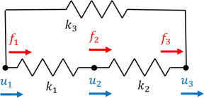
a. Draw the FBD of each spring. Call the spring forces fk1, fk2, fk3
b. Draw the FBD of each mass in terms of the applied forces and spring forces and write the equation of motion for each mass (![]() = ma)
= ma)
c. Using Hooke’s law, convert the equations from (b) into equations in u and ü, where each overdot represents a derivative with respect to time
d. Convert the equations above into matrix equations. Write out each matrix. Because we have 3 DOF, we should have 3x3 stiffness [K] and mass [M] matrices, and 3x1 acceleration {![]() } displacement {u} and load {f} vectors.
} displacement {u} and load {f} vectors.
2. Now create the stiffness matrix from P1 using the matrix assembly process:
a. Write the 2x2 stiffness matrix for each spring (local element coordinates - see CH3 LW notes)
b. Write the 3x3 stiffness matrix for each spring (global coordinates - see CH3 LW notes)
c. Show that [K] from (1d) is equal to the sum of the 3x3 matrices in (2b)
3. Assemble and solve the system in Matlab:
a. Create a folder for your work: ‘\MEMS424\HW1’ or something similar. Create a new script within that folder called ‘mems_424_hw1_p3.m’ or similar. Note that spaces are not allowed, and you cannot start a file or variable name with a number.
b. There is a template that you may use to create the solver. You can copy/paste from this template, or you can edit it directly. Solve the system by competing the template.
c. When you are finished, publish your Matlab code to PDF. Under the ‘PUBLISH’ tab, go to Edit Publishing Options, then set the Output file format to ‘pdf’ . Click the Publish button.
4. Using the UNCONSTRAINED stiffness matrix obtained in problem 3,
a. manually do Gauss elimination on the 3x3 stiffness matrix augmented with a (nontrivial) balanced load – you choose the loading. Show that this leads to a ‘free parameter’ – if you have a row of zeros, you have one free parameter. All other unknowns can be solved in terms of this parameter.
b. manually do Gauss elimination on the 3x3 stiffness matrix augmented with a (nontrivial) unbalanced load – you choose the loading. Show that this leads to an impossible equation 0 = nonzero_constant. No solution is possible.
5. Copy your problem 3 script and call it ‘mems_424_hw1_p5.m’ or similar. We will use most of that script, but alter it to solve for natural frequencies. Assign the following mass values m1 = 10kg, m2 = 20kg, m3 = 15 kg. Create the diagonal mass matrix using the diag() command in Matlab. Comment out or delete the code that solves for displacements.
Hint, here is another way to create constrained matrices in Matlab:
nDof = 8; % assume 8 degrees of freedom, for instance
fixedNodes = [2 5]; % we want to fix nodes 2 and 5
freeNodes = 1:nDof; % this is all the nodes, we will need to remove some… freeNodes(fixedNodes) = []; % remove nodes that are fixed from this list Kc = K(freeNodes, freeNodes);
Mc = M(freeNodes, freeNodes);
a. Find the 2 natural frequencies of the system when mass 1 is fixed. No need to show code, just give the frequencies in Hz.
b. Find the 3 natural ‘frequencies’ of the system if no constraint is applied. What does it mean if one of these frequencies is zero?
c. Answer these questions: Did we use the load vector in solving for the natural frequencies? Can you think of cases where applied loads would affect the natural frequencies?
6. Copy your problem 5 script and call it ‘mems_424_hw1_p6 .m’ or similar. We will use most of that script, but alter it to solve for dynamic response.
a. Fix node 1. We should now have 2 free nodes (2 and 3) with forces of 1000N and -200N applied to them.
b. Create parameters for the initial and final time of the simulation: t0=0; tf = 3;
c. Create a vector of zero initial conditions. Because we are solving a 2nd-order system, we need initial conditions for position and velocity. Something like this would work:
y0 = zeros(2*numel(freeNodes),1); %just a column with 4 0s
d. Create a load vector for the state space equations. To be general, we could do it like this:
p = [fc;zeros(numel(freeNodes),1)];
e. Create the block matrices shown on page 13 of the LW notes. Here is some example
code to create the block matrix A:
Z = zeros(size(Kc));
A = [Mc, Z; Z, -Kc];
We will assume mass-proportional damping with a = 0. 1 and F = 0.001, create parameters ‘alpha’ and ‘beta’ in the parameters section (not down at the bottom where they will be buried).
C = alpha*Mc + beta*Kc;
Create the B matrix as a block matrix of C, Kc, and Z matrices.
f. Run your code so far and verify by inspection that A and B are symmetric. Alternately, confirm that A-A’ is a matrix of zeros as is B-B’ (the apostrophe is a transpose in Matlab)
g. Create an anonymous function. There are multiple ways to do this, but this is one: dydt = @(t,y)A\(-B*y + p);
This might be an inefficient way to do this, but we wont worry about that for now.
h. Finally, call an ode solver and plot your results. We will use the trusty Matlab ode45(): [t,y] = ode45(dydt,[t0, tf], y0);
i. We will plot the motion of the two masses. Because of the way that we set up our state-space equations, these are the last two elements of our
solution vector (y3 (t), y4 (t)).
plot(t,y(:,[3 4]))
j. Add axes and units for your plot. Add a grid. Add legends for ‘u1’ and ‘u2’ . When it looks good to you, publish your code to pdf using the Publish button.
2023-01-31