Question 1 [2 + 2 + 2 + 4 + 1 + 1 + 3 + 1 + 1 + 5 = 22 marks]

a) Shown below is the table illustrating the number of employees from two different

depart5ments: Production and Engineering (P&E) ad Purchasing by gender and the

educational attainment (in years).

Use Exhibit 1 below to answer the following questions.

Using the two pivot tables in Exhibit 1,

(i) Calculate the proportion of the female and the proportion of the male employees from the P&E department. Show all workings to 4 decimal places.

(ii) Similarly, calculate the proportion of the female and male employees from the Purchasing

department. Show all workings to 4 decimal places.

(iii) From part (i) and (ii), compare the percentage of the employees from the two departments.

b) Next, we want to examine the variable of employee’s experience and the distribution of employees. Pivot tables (Exhibit 2) below show the employee experience from P&E and Purchasing departments.

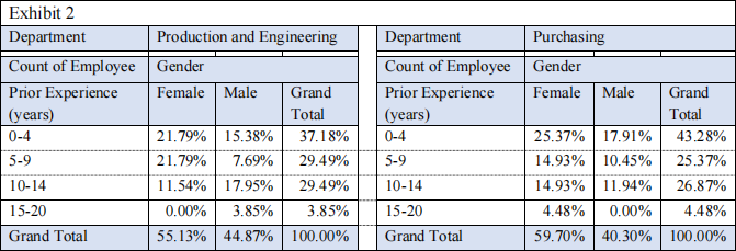
Based on the above reported probabilities, discuss how the employees prior experience affects the distribution of the employees as their experience increases. Give examples.

c) The pivot table below (Exhibit 3) gives the employee’s prior experience by employees’ gender for all company’s departments.

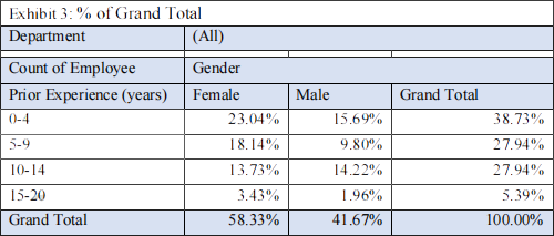
From this Exhibit 3, answer the following questions.

(i) What does the value 5.39 present?

(ii) Explain the meaning of the value 9.80%.

d) Below is a chart of showing the distribution of employees’ salaries by their prior experience for all departments.

Exhibit 4.

For the following questions, refer to above Exhibit 4.

(i) Does the prior experience really matter in terms of employee’s salary? Discuss giving the evidence in terms of values and the percentage estimates.

(ii) Which range of years of experience has the highest percentage of group of annual salaries?

State the salary group and the percentage as well.

(iii) Which is the most salary group with the most years of experience?

What percentage is that group?

e) The pivot table below (Exhibit 5), examines the distribution of employees’ salaries by their prior experience for all departments.

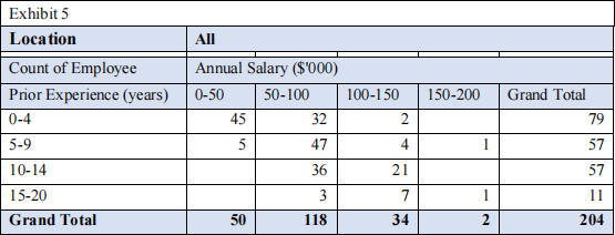
Here we want to find out if the employees’ prior years of experience is independent of their annual salaries.

Specifically, using Exhibit 5, establish if “Salaries=0-50” is independent of “Experience=0-4”

In support of your explanation, write down the required probability statements supporting.

Question 2 [3 + 2 + 2.5 + 4 + 5 + 3 + 4 = 23.5 marks]

a) Summary statistics and the distribution of the employees’ salaries for all departments are provided below (Exhibit 6).

Exhibit 6

Exhibit 7

(i) What type of chart given in the Exhibit 7

Give three essential items/elements that will improve this type of chart.

(ii) Using Exhibit 6 and 7, describe the shape of the “Annual Salaries” of the employees.

(iii) It is hard to state the mode in the continuous data. However, from Exhibit 7 what would be

the annual salaries modal class?

Obtain the percentage of this modal class. Show your calculations.

(iv) Using Exhibit 7 interpret in context the central tendency of the annual salaries.

(v) To describe the variation of data, we use Range, interquartile range (IQR) and coefficient of variation (CV).

From Exhibit 7, illustrate how we calculate Range, IQR and CV

Give interpretations for two of any of these three measures.

b) To use the Empirical Rule we assume the data is approximately normally distributed. If this rule is applied to the employee’s annual salaries, use Exhibit 7 to answer the following        questions.

(i) Calculate the annual salary that 2.5% of employees who receive a salary equal to or lower than this value. Show your workings.

(ii) What is an approximate probability of a randomly selected employee who receive a salary

between $41,022 and $101,527?

Show your workings.

Question 3 [1 + 3 + 4 + 2.5 + 2 + 6 = 18.5 marks]

a) Using the data “US Income.xlsx” let us define the following variables:

Income (Per Year) = Individual annual income ($).

Female = 1 if an individual is a female and 0 if a male

Proportion = values of 1’s

Using excel we obtain the regression of variable the “Female” on the variable “Proportion” . The out is given below, Exhibit 8.

Exhibit 8

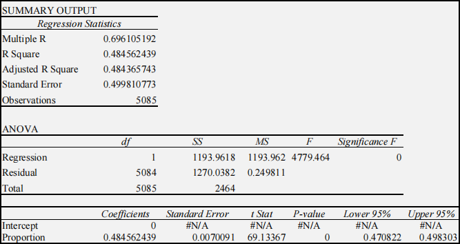
Use the above Exhibit 8 to answer the following question

(i) State and interpret the coefficient of the “proportion” variable.

(ii) Calculate the male proportion and compare it with the female proportion.

(iii) State and interpret the 95% confidence interval for the proportion variable in Exhibit 8 in context.

b) (i) As we are dealing with the sample proportion, explain the concept of “repeated sampling” and give a “mathematical” interpretation of the 95% confidence interval in Exhibit 7.

(ii) Explain what effect the sample size being decreased will have on the confidence interval in

Exhibit 1 if all other factors are assumed constant.

Explain your answer.

(iii) What would happen to the confidence interval in Exhibit 1 if we instead constructed a 90%

confidence level given that all other factors remain constant?

Explain your answer.

c) Next, we use Excel to obtain a regression of Income (Per Year) on Female. The output is given below in the Exhibit 9.

Exhibit 9

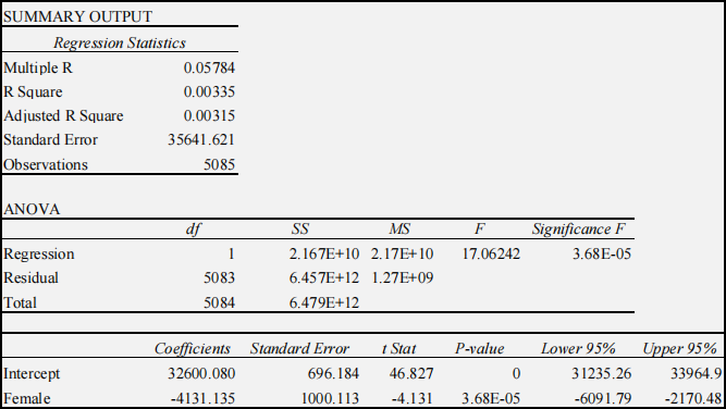
Use the above Exhibit 9 to answer parts i, ii & iii

(i) State and give an interpretation of the intercept coefficient.

(ii) State and give an interpretation of the slope coefficient.

(iii) Carry out a hypothesis test to establish if the difference between the male and female annual

incomes is significant at 1% level of significance

Use the p-value approach and show all the steps.

Question 4 [3 + 3.5 + 4.5 + 2.5 = 13.5 marks]

We want to explore the variables that might influence the amount the customer spends at HyTex on purchases. We define the following variables:

Y variable:

AmountSpent = Total amount spent on purchasesfrom HyTex ($).

X variables:

Male  = 1 if a person is a male and 0 iffemale.

a) (i) First, carry out a correlation matrix of variable of “AmountSpent” on the above variables” . Name that Exhibit 10.

Exhibit 10

(ii) From Exhibit 10, which variable have the most influence and the least impacts on the

“AmountSpent”?

Sate and interpret one of these two values.

b) Excel is used to regress “AmountSpent” on Male, OwnHome, Married, Salary, Children, and Catalogues. The output is given below in the Exhibit 11.

Exhibit 11