Ec5040/Ec5330 Assessed Computer Exercise
Hello, dear friend, you can consult us at any time if you have any questions, add WeChat: daixieit
Assessed Computer Exercise
Learning Outcomes: This exercise is intended to assess your working knowledge of many of the topics covered in the first term and counts for 15% of your total mark for Ec5040/Ec5330.
Load up your answers to the Computer Assignment turnitin link on course moodle page by 5pm on Friday 20th January 2022
Your answers should consist of Stata output and some explanatory text. Download your Stata output into a Word file and add some explanatory text (the better the explanatory text the higher the marks will be)
Hint: Stata output from the screen can be copied directly into Word by highlighting the relevant output and then copying into a Word document. The “Courier New” font with an 8 or 9 point font size works best. See the Guide to Using Stat on Week 1 of the course moodle page
Make sure you write your student number at the top of your answer document (the one that starts with 100……
Instructions
Read in the data set comptest_2022_ `i’.dta from the Ec5040/5330 moodle site folder marked “computer test data” in the Assignments Folder.
(The `i’ is the same number you were assigned for the mid-term take home)
This is a 2-period panel dataset on a sample of around 1,400 working individuals in the United Kingdom who were asked about their wages and various socio-economic characteristics
when aged 33 and then again aged 42.
The dataset contains the following variables:
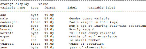
The idea is to estimate the determinants of log hourly wages where one of the right hand side variables may be endogenous.
Consider the following model
LnWage = b0 + b1yearsed + b2exper + b3exper2 + b4worksft + u
1. Summarise the variables in the regression model
(comment on the means of each of the variables in your data set)
Do an OLS regression of the model above for all women aged 42 only
(you will have to generate the experience squared and the log of hourly wages variables yourself and work out how to select only the subset of women who are aged 42 for the regression)
Interpret your estimates of the effects of years of education and working full-time (10 marks)
2. Now see if you can replicate the OLS estimates and standard errors by writing a Stata program to estimate and display the coefficients and their standard errors. Show the file and the output in your answer.
(Hint: see computer exercises 2, 3 and 7. To help you get the right sample size use the command “keep if e(sample)” at the start of your do file. This will estimate the commands on the same sample size as in the regression in question 1 ) (15 marks)
3. Test for the presence of heteroskedasticity in your model – using the Breusch-Pagan test. Do not use Stata’s automated command, do the test yourself
If heteroskedasticity is found to exist, re-estimate the model taking account of the presence of heteroskedasticity.
Program your own estimates of the robust variance-covariance matrix of the coefficients and compare your answers with those in the Stata output. (20 marks)
4. It is likely that the years of education variable may be endogenous,
(because of omitted variables like ability or because of measurement error or because of interdependence between wages and education).
Assuming that measurement error exists estimate the bounds in which the true effect of years of education lies for the simple 2 variable model for women aged 42
LnWage = b0 + b1yearsed + e (10 marks)
5. Write a computer program to take 200 (different) random samples of size
a) 400 of the women aged 42 from your data set
b) 25 of the women aged 42 from your data set which estimates the model
LnWage = b0 + b1yearsed + b2exper + b3exper2 + b4worksft + u
for women aged 42 by OLS
Copy the program into your answer document and show the plot of the resulting distribution of estimates on the coefficient years of education.
Comment on what you find (15 marks)
Hint look at the do file “bsample.do” in week 3 of the course moodle page and cex9.do in week 9. You will have to change the variable list and the sample commands and the name of the directory and file path
6. Since years of education is endogenous the data set contains two possible instruments for education
i) a variable measuring the age at which the individual’s mother left full-time education, (mumlfte)
The idea is that mother’s education is likely to affect the level of their child’s education but
have no direct effect on their child’s wages
ii) A variable for father’s weight (dadweight).
The idea is that weight is correlated with wealth and parental wealth is known to affect children’s education levels
Compare the IV estimates and the associated standard errors on the coefficient on education for the model estimated at age 42
using
i) The mother’s education instrument
ii) The father’s weight instrument
iii) both instruments together
You will have to work out which variables to enter in the stata “ivreg” command and in which order
Give reasons why your answers differ across the specifications (15 marks)
7. See if you can adapt your program in question 5 to include additionally a distribution of estimated effects of years of education from an IV regression of the model using mother’s education as the instrument for years of education using the 90% sample.
Plot the resulting distribution of IV estimates alongside the distribution of OLS estimates. Comment on your results
2023-01-18