ECE 364 Project: Image Blending & Morphing
Instructions
Work in your Lab12 directory, and you can copy the data files into that folder.
You must meet all base requirements in the syllabus to receive any credit.
Remember to commit & push the required file(s) to GitHub periodically. We will only grade what’s been pushed to GitHub!
Do not push to GitHub any file that is not required. You will lose points if your repository contains more files than required!
Make sure you file compiles. You will not receive any credit if your file does not compile.
Name and spell the file, and the functions, exactly as instructed. Your scripts will be graded by an automated process. You will lose some points, per our discretion, for any function that does not match the expected name.
Make sure your output from all functions match the given examples, within acceptable tolerance. You will not receive points for a question whose output mismatches the expected result.
You can use any module from the Python Standard Library, but, aside from the libraries described in the document, you cannot use any external library.
This is the first of two phases for the course project for ECE 364.
This is an individual project. All submissions will be checked for plagiarism.
Make sure you are using Python 3.7 for this project.
Introduction
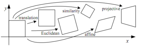
Combining two images into one, or image blending, has many applications in image processing. One application that utilizes image blending is morphing { a special effect in motion pictures and animations that changes (or morphs) one image or shape into another through a seamless transition1. While there are many ways to perform morphing, we will use a combination of linear projective transformations to achieve our goal. A projective transformation is a process that applies translation, rotation and scaling to a plane to transform it into a different plane. Figure 1 shows different transformations applied to a plane2. This process works by using a non-singular (invertible) 3 × 3 matrix, referred to as the projection, or the transformation, matrix, and applying it to the plane coordinates to transform it from one system to another. In this project, we will concentrate on one type of those transformations, the ‘’Affine Transformation". You will apply affine transformations to different sections of images to produce the effect of non-linear image warping.
Derive different affine transformation matrices for different sections of the image, based on point correspondences between source and target images.
Apply the obtained transformations between the images, and blend two images to have a visually appealing result.
Blend two images, with varying weights, to generate a morphing video.
Preliminary Information
Python Modules
This project utilizes three popular Python modules: numpy.
scipy.
imageio.
These modules have excellent documentation and community support, and while this project will use basic functionality from these modules, you are strongly encouraged to investigate them extensively, as you almost surely will need to work with them in any Python-related scientific code-base. These libraries are already present in the computer system and are accessible in PyCharm. Your work in this project will primarily be with the object ndarray from the module numpy.
Please note the following:
You should import numpy is as: import numpy as np
You will need to perform all mathematical operations using numpy types, like np.uint8 and np.float64, as opposed to native Python types integers and floats, to reduce numerical errors.
There are multiple ways to carry out the same operation in numpy, but some are fast and some are very slow. Choosing the wrong method can significantly slow down your development and performance.
Based on many factors related to carrying out mathematical operations in the code, your results might have slight numerical variations from the reference images. Your images will be accepted as long as they look \visually" identical to the human eye.
Accessing Image Data
In its simplest form, an image is a 2D Array of pixels. (Review the module imageio for information on loading an image into a 2D array.) In gray-scale images, a pixel is represented by a single byte, i.e. it takes an integer value between 0 and 255, while in color images, each pixel is represented by three bytes, one for Red, Green and Blue respectively, and each one can take a value between 0 and 255 as well. The colors in the image are also referred to as “channels" or “bands". Without loss of generality, we will be discussing how to work with gray-scale images.
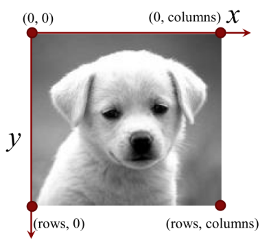
Figure 2: An image can be accessed either by row and column indices, or by x and y coordinates.
Since the mathematical foundation of affine transformation is based on plane-to-plane transformation, it is useful to think of an image as a surface on a xy-plane, where at each specific (x; y) coordinates you get f(x; y) which corresponds to the pixel value at the [x; y] indices. As shown in figure 2, the convention is for the origin to be in the upper-left corner of the image, which helps align the x and y coordinates with the row and column indices of the image such that x is the column value, and y is the row value.
While image values are defined at integer indices, treating the image as a surface allows us to access the image at non-integer coordinates, like at x = 3:5; y = 2:75. We can obtain the image value at such locations by utilizing 2D interpolation to approximately calculate that value from its 4 neighbors. There are different mathematical approaches to performing 2D interpolation, the simplest of which is bilinear interpolation3. You may use any method for bilinear interpolation, whether from libraries you are working with, as in the functions:
scipy.interpolate.RectBivariateSpline()
scipy.interpolate.interp2d()
scipy.ndimage.map_coordinates()
or whether you implement your own. (If done carefully, your own implementation may give you a performance boost.) Please refer to the scipy documentation on how to use these function.
Affine Transformation Matrix and Homogeneous Coordinates
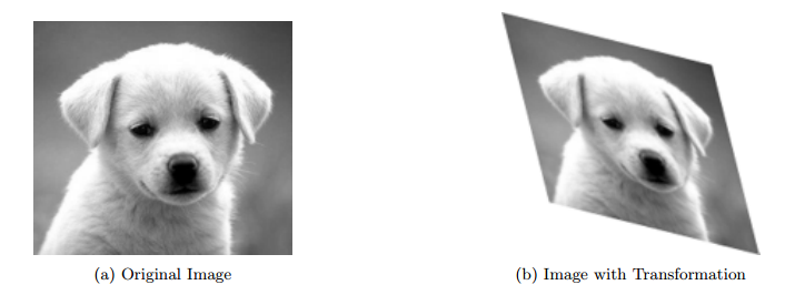
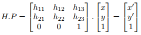
Given a transformation matrix, H, we can transform an image from one plane to another, as shown in Figure 3. Note that this transformation process is invertible, i.e. if we use the matrix H to transform image A into image B, we can use the inverse matrix H-1 to transform B back into A4. In order to apply a transformation to a given image, we are going to utilize homogeneous coordinate, which simply augments a point in a plane to be a point in space by adding a third coordinate value, and setting it to 1.By doing that, each point becomes a 3 × 1 column vector at which we can multiply it with the matrix to perform the transformation. For example, if we pick any point P = (x; y) in the original image, we can transform it to P 0 = (x0; y0) in the target image using the matrix H as follows:
To avoid this issue, we use the idea that affine transformation is an invertible process, and we iterate over the points in the target region instead, to get the source point using the inverse matrix:
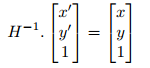
By doing so, we can restrict our access in the target image to go over the integer indices (x0; y0), and we obtain the point (x; y) from the source image, which we can read, to assign it back to the target. If the source point (x; y) contains non-integer values, we can simply use 2D interpolation to obtain the desired value, as explained in the previous section.
One other thing to keep in mind is that performing matrix algebra is better done using float values (like np.float64). However, when assigning values to an image, it has to be converted to an 8-bit unsigned integer type, np.uint8. If you simply perform the assignment, numpy will perform a truncation over the values. Hence, it is better to manually apply a rounding operation, (using np.round(), and not Python’s built-in round() function,) before you assign a float value to an integer value.
Identifying Points in a Region of Interest
Transformations can be applied to the whole image, as shown in Figure 3, or to a subregion of an image, often referred to as Region-of-Interest, or ROI. The ROI can be a polygon of any form, but in this project, we will only be dealing with triangular ROIs, since both the source and target will be triangles. There are different techniques5 to obtain the indices of all the pixels that lie within a triangle’s vertices. You can either choose an implementation that is already provided, or implement one yourself.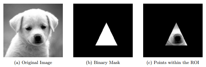
Matrix Computation from Correspondences
In the previous sections, we described how to \apply" a transformation to an image, or a region of interest within an image, given that the transformation matrix is already provided. But, how do we obtain that matrix? Without delving too much into the projective geometry theory, computing an affine transformation matrix is simply done by solving a system of equations using linear algebra. In order to construct the system of equations, we need to identify three-point correspondences, as shown in Figure 5, where each correspondence is a pair of points.Intuitively, this process aims to find the matrix that transforms the point (x1; y1) from the source image to the point (x0 1; y10 ) in the target image, the point (x2; y2) to the point (x0 2; y20 ) and so on. The mathematical derivation of this process is beyond the scope of this project, but the implementation is straightforward.
Each point pair will be used to provide us with the following two matrices:
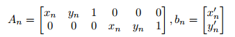
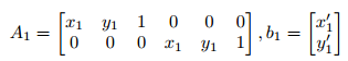
For example, the correspondence pair (x1; y1) and (x0 1; y10 ) will give the matrices:
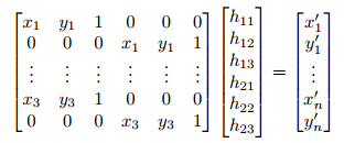
h = np.linalg.solve(A, b)
Finally, we rearrange the column vector into the affine projection matrix H:
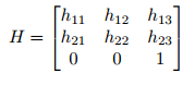
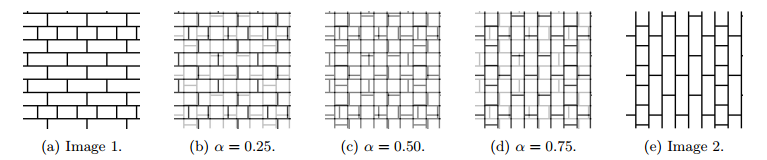
Image Alpha Blending
A common technique to combine two images I1 and I2 with different weights is alpha blending, where α is a value between 0 and 1 that controls how much of each image we are adding in the final blended version. When α = 0, we are retaining the first image, and nothing from the second, and when α = 1, we are retaining the second image and nothing from the first. For all other values of α, the blended image, B is calculated as: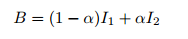
Implementation Details
Create a Python file named Morphing.py, and do all of your work in that file. This is the only file you need to submit for this phase. You can write any number of \classes" and helper functions in this file, but DO NOT CREATE ANY MODULE VARIABLES.Notes:
The requirements below represent the public interface that your classes should conform to. You will need to implement additional functions, and include other member variables, to simplify your code. Otherwise, your methods will become impossible to read and debug.
Modify the .gitignore file in your Lab12 folder to contain the following lines:
*
!.gitignore
!Morphing.py
!README
Point Data Loading
Write a function called loadTriangles that takes in the full file path of the text file containing the (x; y) coordinates of a list of points. This module function should return a list of instances of the Triangle class. (Note that the Delaunay triangulation can be used to obtain the triangles from the points of interest.)Triangle Class
Implement the Triangle class that contains the information about a triangle in the xy-plane.Member Variables:
vertices: A 3 × 2 numpy array of type float64 containing the vertices of a single triangle in the xy-plane.
Member Functions:
Initializer: Initializes an instance through providing the required argument vertices. Raise a ValueError with an appropriate message if the input argument does not have the expected dimensions or if it is not of type float64.
Write a member function called getPoints that takes in no arguments, and returns an n × 2 numpy array, of type float64, containing the (x; y) coordinates of all points with integral, i.e. integer-valued, indices that reside inside the triangle.
Morpher Class
Implement the Morpher class that performs all morphing operations.
Member Variables
leftImage: An m × n numpy array of type uint8 containing left, or starting, image of the morphing process.
leftTriangles: A list of Triangle instances containing the triangles that belong to the left image.
Member Functions:
Initializer: Initializes an instance through providing all of the member variables in order, i.e. leftImage, leftTriangles, rightImage and rightTriangles arrays.
Notes:
- Verify that all input arguments are of correct types, and raise a TypeError with an appropriate message otherwise.
- Do not hard code the size of the image passed anywhere in your code.
Write a member function called getImageAtAlpha that takes in a single float value, alpha, where 0 < α < 1. (Note that for α = 0 you should only get the left image, and for α = 1 you should only the right image.) This function should perform the following for every triangle pair:
- Calculate the middle triangle that corresponds with the given α. Let us call that the target triangle.
- Transform the left triangle onto the target triangle.
- Transform the right triangle onto the target triangle.
Once processing of all triangles is complete, perform a blending between the two target images, and return the result.
Extra Credit
Once you complete the implementation of the required tasks, you might want to implement one or more of the follow tasks. Note that this section cannot be graded if the required implementation is not complete. Moreover, TA help will not be provided in this section.Generating a Morphing Image Sequence and Video
Add a member function called saveVideo to the Morpher class that takes in the following arguments:
targetFilePath, a string containing the full path of the target video file, with extension .mp4.
frameCount, an integer, greater than or equal to 10, representing the desired number of video frames. Note that this count includes the left image, where α = 0, and the right image, where α = 1.
frameRate, an integer, greater than or equal to 5, representing the frame rate of the video.
includeReversed, a Boolean flag, defaulted to True, indicating whether the generated frames should be duplicated, but in reverse, giving a final frame count of (2 * frameCount). If the flag is False, then the final video has a frame count of frameCount only.
Notes:
The generated video may have slight size differences from the individual frames, and its file size can vary based on your generation method.
The easiest way is to use ffmpeg tool to generate the desired video.
The video is not expected to be an exact binary match to some reference. It will be checked manually by the TAs for some properties.
You may create intermediate images for the video generation, but they must be placed in temporary folder outside your code folder (like /tmp/
Working with Color Images
The required part of the project only deals with the images being in grayscale. In this part, create the ColorMorpher classes that performs the same functionality over color input images. This class must inherent from the Morpher class, and must have the same interface, i.e. the same member functions and function signatures. While not required, and will not be checked, there should be no duplicate code between the base class and the subclass.Performance
As mentioned earlier, working with Python and the numpy library can offer multiple ways to tackle the same requirement. In this part, you will need to consider creating a robust and performant application, and not just that which satisfies the functionality. If you paid attention to designing and implementing a performant application, the execution time gain can be measurable. For this requirement, you will be provided with execution times for certain tasks, and your code should achieve comparable times.Personal Morph
Use your code to create a video of a morph using your own mug shot as the starting image, and your choice of the ending image: a celebrity, an animal, a solid object, etc. Both images should be of the same size used in this project, i.e. 1080 × 1440, and should use a large number of point correspondences. The amount of points given in this part will be determined by the quality of the morphing, as judged by the TAs.
2019-04-09