STATS 330

STATISTICS

Advanced Statistical Modelling

(Time allowed: TWO hours)

INSTRUCTIONS

• Attempt ALL 3 questions.

• There are a total of 80 marks for this examination.

• There is a list of useful formulae on the last page of this exam.

1. [35 marks]    The data described below show the free-throw results obtained by the Los Angeles Lakers player Shaq O’Neal in 23 NBA play-off games in the year 2000. (For those unfamiliar with basketball, a free throw is when a player is allowed to take an unopposed shot at the basket from the free-throw line. Thus in game 1, O’Neal attempted 5 free throws, 4 of which were successful.) People are interested in whether the number of attempted free throws and the proportion that were successful changes as the play-offs progressed (i.e. with increasing game number).

The data in the file Shaq.df consists of:

game    the game number

n          the number of free throws

s           the number of successful free throws.

Consider the plot and fitted model below:

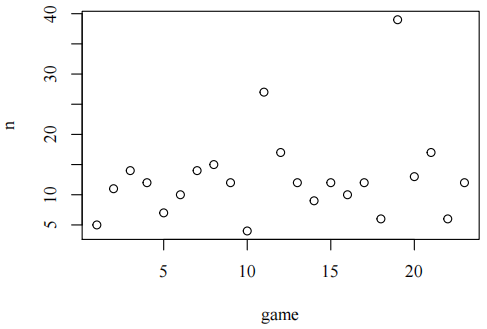
(a) For n.mod1, what is (i) the assumed relationship between game and the number of free throws n, and (ii) the assumed distribution of its response value? [5 marks]

Consider the following code:

(b) Using this output explain why we prefer n.mod2 over n.mod1 in terms of model adequacy. [5 marks]

Consider this negative binomial analysis of these data:

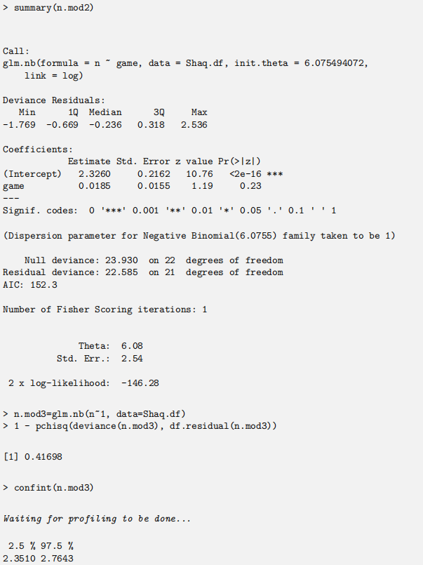
(c) The estimate and its standard error associated with the variable game (from the model n.mod2) are 0.0185 and 0.0155, respectively. Explain how we obtain the z value of 1.19. [5 marks]

Consider another negative binomial analysis of these data:

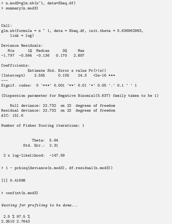
(d) For model n.mod3 calculate the value of the Pearson residual associated with the first play-off game. [5 marks]

Consider the following analysis of the proportion of successful free throws by O’Neil over this play-off season.

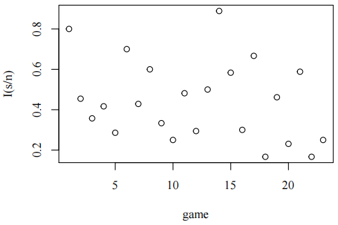
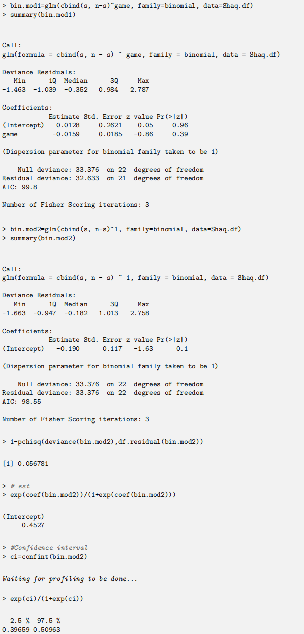
(e) It appears there is some evidence that these data are not consistent with a Binomial distribution. This observation is based on using a chi-squared distribution to approximate the sampling distribution of the residual de-viance. Explain why the use of a chi-squared distribution may not be valid in this case. [5 marks]

With the above comment in mind, the following simulation was performed:

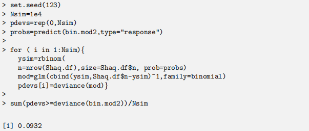
(f) What do we conclude from the above analysis? Explain briefly. [5 marks]

Assume the model bin.mod2 can be used for interpretation.

(g) Write a brief executive summary about the number of free throws and their success rate for Shaq O’Neal in these play-offs. [5 marks]

2. [20 marks]    Roberts and Foppa (Vector-Borne and Zoonotic Diseases, 2006, 6, 1–6) used Poisson regression to model the occurrence of West Nile virus (WNV) in horses. WNV is a disease that attacks the central nervous system and its effects can be fatal. Birds are the most commonly affected animal but WNV also affects mammals including horses and humans. WNV is spread mainly by mosquitos, with birds being the primary hosts for the virus. Typically, bird mortality due to WNV precedes human and equine infection and thus dead bird surveillance is used to monitor the risk to human and horse populations. Es-sentially, people are asked to report cases of dead birds which are then collected and tested. As population increases it is expected that more dead birds will be reported and thus the number of positive tests will be higher. To compensate, the “positive bird rate” (the number of dead birds that tested positive for WNV divided by the population of the county) is used as the explanatory variable of main interest.

Data collected for 25 counties in South Carolina, USA in 2003 were used to fit a model that involved the following variables:

equine: The number of cases of WNV in horses (response variable).

farms: The number of farms in the county (offset variable).

PBR: The positive bird rate per 10,000 population (explanatory variable of main interest).

density: The population density recorded as people per square mile (explanatory variable).

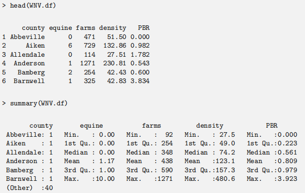
The following output shows the first 6 observations in the data set and a summary of the variables:

Consider the following negative binomial regression model:

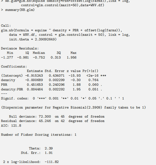
(a) The main purpose of this model was to relate the number of cases of WNV in horses equine to the positive bird rate PBR.

i. The model includes log(farms) as an offset. How does this affect the interpretation of this model?

ii. The model includes density as an explanatory variable that interacts with PBR. As a result the relationship between equine and PBR depends on the level of density. Compare the relationship between equine and PBR for a county with a density of 100 people per square mile to a county with a density of 200 people per square mile.

iii. Based on this model, what is the fitted value of equine for Abbeville county? Note that the values of the explanatory variables for Abbeville are given on the previous page. [6 marks]

(b) Consider the following output

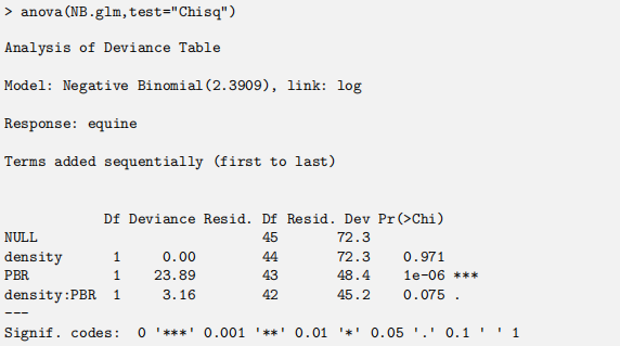
i. The output from anova() gives a different p-value for density:PBR than does the output from summary() even though they are both testing the hypothesis that the interaction is not needed in the model. Explain why this occurs.

ii. Suppose that you wish to test the hypothesis that the interaction is not needed in the model without assuming that the change in deviance will have a chi-squared distribution. Explain how you would do this. [7 marks]

(c) Suppose that this model is to be used to predict cases of WNV in horses in other counties. Explain how a realistic estimate of the MSPE (mean square prediction error) could be obtained. [7 marks]

3. [25 marks]    In Lecture Handout 16, data concerning academics at the Uni-versity of Washington were used as an example for causal analysis. For this question, we are going to consider the following subset of the variables from that example:

gender: F (female) or M (male).
deg: highest degree is a PhD (PhD), Prof (a professional degree) or other (any other type of degree).
field: is Arts (visual and performing arts), Prof (medicine, law, nursing . . . ) or other (any other field).
startyr: year of first employment.
rank: in 1995 is Assist (assistant professor), Assoc (associate professor) or Full (full professor).

admin: is 0 (no extra pay for admin duties) or 1 (extra pay for admin duties).

Consider using these data to investigate the causal impact on admin of the other variables. Assume that the following causal diagram as being appropriate for this situation.

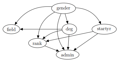
Based on this diagram it can be deduced that:

● rank, gender, deg and startyr have direct effects on admin and to esti-mate these direct effects we should use a model that contains rank, gender, deg and startyr as explanatory variables.

● to estimate the total effect that gender has on admin, we should use a model that just uses gender as an explanatory variable.

(a) What model would you use to estimate the total effect of deg on admin? Explain your choice of model. [5 marks]

(b) The following logistic regression model can be used to investigate the direct effects of rank, gender, deg and startyr on the chances of an academic receiving extra pay for administrative duties (admin).

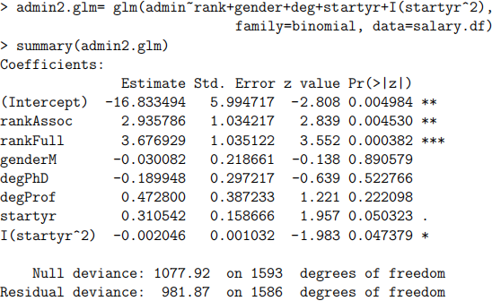
i. Use this model to estimate the difference in the log(odds) of receiving extra pay for administrative duties between an academic whose highest degree is a PhD and an academic who has a professional degree (given the levels of the remaining explanatory variables are fixed).

ii. Given that gender and deg are set to their baseline levels, what is the estimated probability that a full professor with startyr= 70 receives extra pay for administrative duties?

iii. Does this model suggest that male academics are more apt to receive extra pay for administrative duties than female academics (given the levels of the remaining explanatory variables are fixed)? Explain your answer. [9 marks]

(c) The logistic model that just has gender as an explanatory variable can be used to investigate the total effect that gender has on admin.

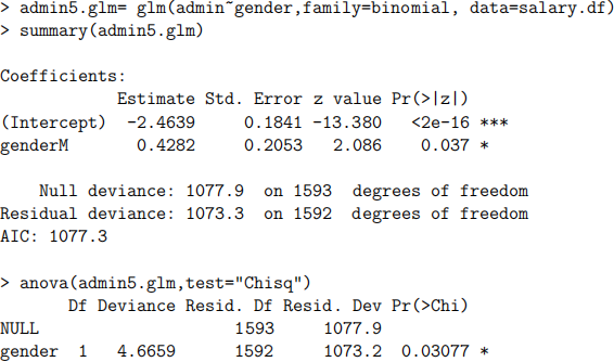
Based on this output, describe the total effect that gender has on admin. [5 marks]

(d) Using the results from (b) and (c), describe the nature of the relationship between gender and the probability that an academic receives extra pay for administrative duties. Your explanation should be understandable for someone who is not familiar with the terms “direct effect” and “total effect.” [6 marks]

Some Useful equations

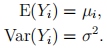
If  ~ Normal, then

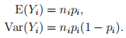
If  ~ Binomial, then

If  ~ Beta − Binomial, then

Here, ρ will appear as rho in any R-output. (Also, sometimes, called θ (or theta in R)).

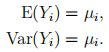
If  ~ Poisson, then

If  ~ negativebinomial, then

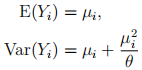
Here, θ will appear as theta in any R-output.

For model fitting a model mod: where k is the number of parameters used in describing the model and is the log likelihood.