For this assignment:

– You may work in groups of up to three.
– There is a version of cvx available for python, called cvxpy. You are welcome to do this assignment in python if you would prefer.

Background

In this homework, you will look into “structure estimation” using our convex optimization tools and Gaussian graphical models. The motivation behind Gaussian graphical models is as follows: if we have Gaussian random variables and the conditional dependencies between variables are encoded in a graph, the inverse of the covariance matrix will have zeros for pairs of variables that  are not connected in the graph. For instance, if the relationships between variables X, Y, and Z are as depicted in the following graph:

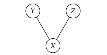
then the inverse of the covariance matrix for (X, Y, Z) will be of the form , where * denotes some non-zero entry. The zeros in the (3, 2) and (2, 3) entries correspond to the lack of an edge between Y and Z in the graph. Long story short, the task of estimating conditional dependencies between variables is the same as the task of estimating zeros in the inverse covariance matrix.

Further, recall that for multivariate normal random vectors, the log likelihood is, up to a constant factor, 

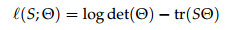
where S is the sample covariance matrix and Q is the inverse of the true covariance matrix.

Assignment

1. Download the data from jfukuyama.github.io/stat710/assignments/hw7.csv. The rows of the matrix are the samples, and the columns are variable measurements. You should have 50 samples and 10 variables.
2. Estimate the inverse covariance matrix using the graphical lasso, that is, solve the following optimization problem:

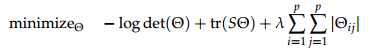
where S is the sample covariance.
For appropriate values of l, this will give you a “sparse” estimate of the inverse covariance matrix , as we want for structure estimation.

You should use the functions log_det and matrix_trace (in the CVXR package).
3. Choose some subset of the elements of the inverse covariance and plot the estimates for a variety of values of l.
4. We would like to pick a good value of l: one way to do this is by cross validation. The idea is to choose the value of l that gives the highest value of the likelihood on a held-out portion of the data.

We will do 10-fold cross-validation.

Choose a range of values of l such that at one end you have a solution with only a few zeros and at the other end you have a solution with nearly all zeros. For each value of l, perform the following:

– Divide the samples into ten groups, and let Ii denote the indices of the samples corresponding to the ith group.

– For each i, fit the model in 1 on the data excluding the indices Ii. Let the estimate of the inverse covariance based on this subset be Qˆ (i).

– For each i, compute the negative log likelihood of the data on the hold-out sample, that is, compute

where S(i) is the covariance computed just on the samples with indices Ii.

– Compute the overall negative log likelihood for the held-out data: -ℓcv = ∑10 i=1 - log det(Qˆ (i)) + tr(S(i)Qˆ (i))

Now you should have values for the negative log likelihood for the held-out data -ℓcv for each value of l. Show the held-out negative log likelihoods against l, and find the value of l with the smallest held out negative log likelihood value.

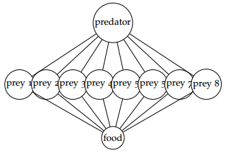
5. It turns out that in this dataset, the first variable is a measure of the abundance of a keystone predator, the second through 9th variables are measures of the abundances of prey species, and the last variable is is a measure of the abundance of a food source. You suspect that the relationships between the variables might be encoded in the following graphical model: 

that is, the predators and prey are have negative partial correlations, the prey and resources have positive partial correlations, and every other pair have zero partial correlation. The interpretation would be that when there is more of the food source, the prey species increase, when there is more of the predator, the prey species decrease, but the prey species do not directly effect each other. 

Perform maximum likelihood estimation under the constraint that the partial correlations between the prey species are zero, that is

minimizeQ - log det(Q) + tr(SQ)

subject to Qij = 0 (i, j) such that i ̸= j, i 2 f2, . . . , 9g, j 2 f2, . . . , 9g

Report your estimate.
6. Obtain bootstrap confidence intervals for the non-zero elements of Q: for some reasonably large number B, perform the following:

– Sample the rows of X with replacement to make a new matrix, X(b), of the same size as X.

– Make a new estimate of Q, Qˆ (b) based on X(b) using the same strategy as in the previous part.

Compute and report the .025 and .975 quantiles of Qˆ ij (b) for each (i, j) pair. These are your bootstrap confidence intervals for Qij.

Submission parameters

Submit two files:

– A pdf writeup containing the answers to the questions.

– A file containing the code you used.