COMP61342: Computer Vision Practical Assignment
COMP61342: Computer Vision
Practical Assignment
Introduction
For this practical assignment you should use Python/OpenCV to develop the code, and present your results as a formal report.
You will find the self-assessment code snippets useful and you are free to use them as part of this assignment.
Each part of the practical will build on the previous parts. You are unlikely to be able to complete the whole assignment immediately, but instead, you should complete it in stages as the relevant material is covered in the lectures.
You will have difficulty if you try to complete the assessment just before the deadline.
You should use the supplied images for your processing and include them in your report.
For ease of marking, please lay out your report in sections using the titles given in this document.
You may want to create separate Python programs for the different parts.
Please submit your results even if you think they are not good enough – you may still receive marks.
Intended Learning Outcomes
By the end of this assignment, you should be able to:
• Implement computer vision code using Python/OpenCV
• Interpret image histograms, especially to aid in thresholding
• Choose combinations of techniques in order to solve a computer vision problem (that is, a computer vision pipeline, or workflow)
• Implement software to create a 3D model from a stereo pair of images
• Perform effects on regions of images depending on their depth into the scene
1 Threshold-Based Segmentation
Figures 1a & 1c shows the images that should be used for this section.
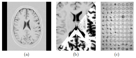
Figure 1: (a) Nuclear Magnetic Resonance image of a brain. (b) Example thresholding of the brain image. (c) Image of a tray in an industrial environment.
1.1 Brain
Figure 1a shows a Nuclear Magnetic Resonance image of the skull and brain. In such images, the distinct tissue types have distinct grey level values.
Create a histogram of the brain image and use it to identify regions of white matter. For reference a white matter segmentation is shown in Figure 1b.
Use a combination of thesholds above and below the white matter peak and some simple image arithmetic to produce your own pixel level binary segmentation of white matter.
If this segmentation was part of automatic computer vision system, it would be beneficial to have an automat-ically selected threshold value. Try using Otsu’s method (cv2.THRESH OTSU) to perform the segmentation. Is the result of any use?
Describe your method and discuss the results.
1.2 Tray
Now attempt the same process with the image in Figure 1c, which was obtained from a CCD camera in an industrial environment. This time attempt to extract the darker contents of each circular cell.
You will notice that illumination artefacts cause position dependant results.
Now filter the image with a large scale smoothing kernel, subtract the result from the original image and try again.
Can you improve upon your initial segmentation?
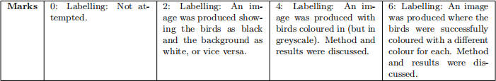
2 Labelling
Use the supplied birds image and label and count the birds.
Each bird that is found should be filled in with a random colour (either onto a black background or onto the original colour image).
Hint: You will probably have a greyscale image that contains a label for each bird (1, 2, . . .). You can use this image to decide which pixels to colour in a separate colour image. You might also use import random, random.randint(0,255).
NOTE You can use an existing labelling algorithm (as discussed in the lectures) but the implementation should be your own.
You can access invidual pixels in an image as follows:
for r in range(img.shape[0]):
for c in range(img.shape[1]):
if img[r, c] == 10:
img[r, c] = 255
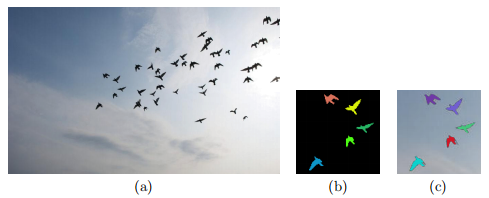
Figure 2: Labelling. (a) Flock of birds. (b) Coloured birds on black background. (c) Coloured birds on original image.
Some of the birds overlap and would be counted as one with a simple algorithm. Pre-process the image to try to separate the overlapping birds. If it does not work as you planned, give details of what you tried.
3 Stereo Imagery
You should use the supplied image pair of photography umbrellas (source: https://vision.middlebury.edu/stereo/data/scenes2014/ – for interest, see the paper ‘High-Resolution Stereo Datasets with Subpixel-Accurate Ground Truth’ by Daniel Scharstein, Heiko Hirschmuller, et al).
Figure 3 shows the image pair and below is the calibration data for them.
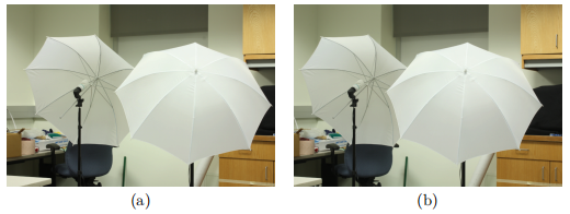
Figure 3: Stereo Pair. (a) Left image. (b) Right image.
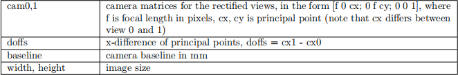
cam0=[5806.559 0 1429.219; 0 5806.559 993.403; 0 0 1]
cam1=[5806.559 0 1543.51; 0 5806.559 993.403; 0 0 1]
doffs=114.291
baseline=174.019
width=2960
height=2016
The key to these parameters is shown in the table below.
However, to make the processing faster, we resized the images to 740 × 505. You might need to take that into account in your calculations below.
You have been supplied with a small program that creates and displays a disparity map (disparity.py). You can use this as a starting point.
3.1 Focal Length Calculation
The paper says that they used two Canon DSLR cameras (EOS 450D with 18–55 mm lens) in medium resolution (6 MP) mode.
This type of camera has a physical sensor size of 22.2 mm × 14.8 mm and in 6 MP mode, the resolution is 3088 × 2056.
Calculate the focal length in millimetres that the two cameras were set to (cam0 is the left camera).

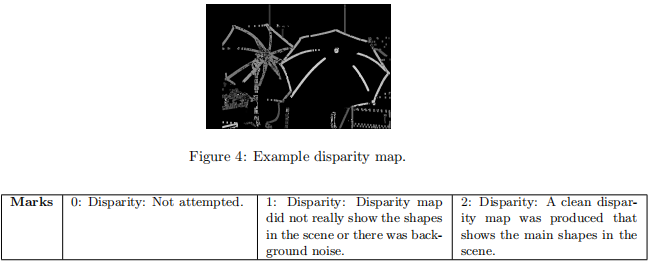
3.2 Disparity Map
Use the supplied program disparity.py as a starting point. The getDisparityMap() function can accept the original images as greyscale or as edge detected images (0 & 255). Try both and see which produces the best result for these purposes.
The getDisparityMap() function returns a floating point image of the same size as the input images with the values corresponding to the disparities. This function takes two additional parameters (number of disparities and block size).
Display an image from the (normalised) disparity map for the umbrella images. Vary the parameters (with Trackbars) until you get an image that looks like the scene without too much noise. Your image might look something like Figure 4.
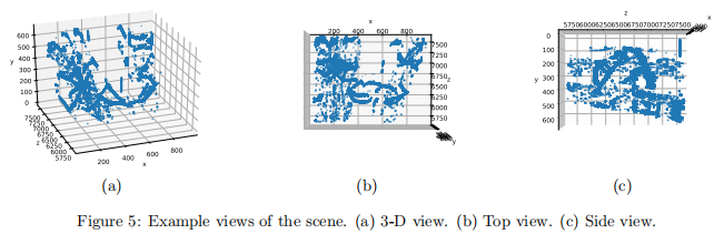
3.3 Views of the Scene
The depth into the scene (Z mm) can be calculated by

where baseline is in mm, and disparity (d), focal length (f), and doffs are in pixels. (You can convert the baseline to metres if you want to get the depth in metres.)
Remembering that pixels represent the light arriving from the scene from different angles, it is possible to calculate the X and Y world coordinates using similar triangles. These can be derived from the focal length, the depth into the scene and the pixel coordinates, x and y.
Loop through the disparity map and calculate the real world coordinates (X, Y, Z) for each pixel in the disparity map. You can do this in the plot() function in the supplied disparity.py, but you will need to pass in some other parameters. Then display a 3D plot of the scene.
Display the resulting data on a 2D plot viewed from above ((X, Z) coordinates) and the side (Y, Z). You might find the matplotlib function ax.view init(elev, azim) comes in useful. (You might find it easier to get the views you want in the matplotlib 3d plot if you swap y and z in the plots.)
Examples are shown in Figure 5. Hopefully, you will getter better results than these if you vary the disparity parameters.
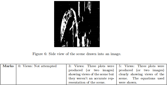
Alternatively, you may decide to create images of your view as in Figure 6. In that case, you do not need to supply a 3-D view, just the top and side views.
4 Selective Focus
Figure 7a shows a mobile phone that has a stereo camera. (For information: It only uses the stereo camera for portraits and will only take the picture if it detects a face – it cannot be used as a general stereo camera.)
The three images in Figure 7 show what you can do with the image after you have taken it. You can blur the background to varying levels and turn the background greyscale.
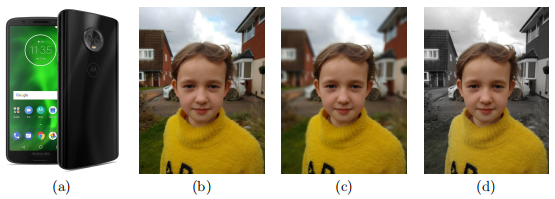
Figure 7: Stereo camera on Moto G6. (a) Phone showing the two cameras on the back. (b) Background blurred slightly. (c) Background blurred more. (d) Background made greyscale.
In this section, you will use the code you have written above to try this yourself (make a copy of your code used for the Stereo section so that you keep both sets of code).
You should use the supplied stereo pair, girlL.png and girlR.png as shown in Figure 8.
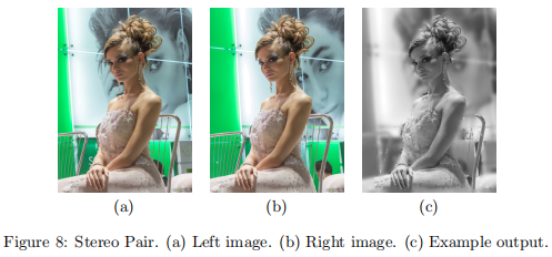
Depth can be approximated from the disparity map (without scale) by
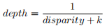
Use a Trackbar on your window to vary k as well as the parameters you did previously. You may find it useful to also display the calculated depth image as well as the disparity image to be able to see a possible segmentation.
The depths can then be scaled to the range [0,255] and image arithmetic performed on this depth image with the original. (How will you decide on which are object pixels and which are background pixels in the depth image?)
Your output can be either of the following:
• A greyscale image with the background heavily blurred.
• A colour image with the background heavily blurred.
• A colour image with the background changed to greyscale.
Hints: Pass greyscale images to getDisparityMap() rather than edge images. Use a larger block size so that more of the image is filled.
You may find that parts of the image have been incorrectly classified (object/background). Small amounts of this throughout the image are acceptable.
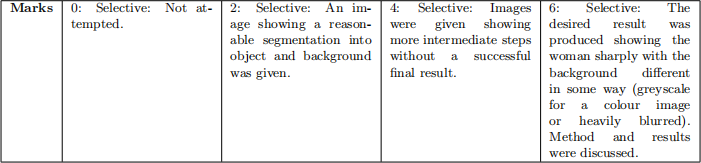
[marks: 25 in total]
Check-list
Have you:
• Created a well-written and well-formatted report?
• Included input, intermediate, and output images with useful labels?
• Chosen a size for your images so that the details can be seen, but not so big that the document covers too many pages (see the images in this document)?
• Included results (e.g. output images) so that report is understandable in itself.
• Included the code in the appendix?
Submit your report as an pdf document on Blackboard.
2021-05-10