MA 9070

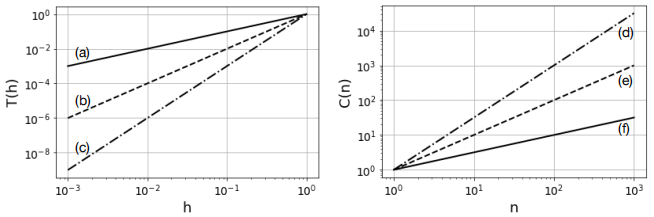
1. a) The plots below show the scaling of truncation error T(h) as a function of grid space h and the computational complexity C(n) as a function of problem size n. For each of the labelled curves, state the big-O form of T(h) or C(n). (No justification needed.) For the truncation error, which curve would be considered to be the best? For the complexity, which curve would be considered to be the best? [12]

b) What is the complexity (time complexity), C(n) = O(npmq ) of the following

for i in range(m):

for j in range(i):

for k1 in range(n):

for k2 in range(k1):

# some fixed amount of computation here [12]

c) State the order of accuracy k for each of the following, where h is grid spacing and ∆t is a time step. No justification necessary.

(i) Truncation error of backward finite difference: . [2]

(ii) Truncation error of centred finite difference: . [2]

(iii) Global error of Euler time stepping for ordinary differential equations: . [2]

(iv) Weak error for Euler time stepping of Brownian motion: . [2]

d) Assume that in pricing a European call option by naive Monte Carlo simulations the variance of the distribution of discounted payoff is 250. Approximately how many Monte Carlo samples N are needed to price the option to an absolute accuracy 0.1, with a 95% confidence level? Make an qualitative sketch of the probability distribution function (pdf) of the discounted payoff and a qualitative sketch of the pdf of the sample mean for sample size N. Since parameter values are not given, sketches need only be qualitative, but you should indicate V , where V is the expected value of the discounted payoff. [16]

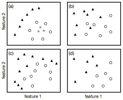
e) The figures below show datasets with two features and either two or three classes. State which subplots (a), (b), (c) and (d) are:

(i) Linearly separable with hard margin. [3]

(ii) Linearly separable with soft margin, but not hard margin. [3]

(iii) Not linearly separable, but nonlinearly separable. [3]

(iv) Not separable. [3]

Answers can include none. No justification required. You only need to state which of (a) - (d) go with each (i) - (iv).

f) State two advantages of mini-batch gradient descent OR state one advantage and one disadvantage of mini-batch gradient descent. You may compare or con-trast with either stochastic gradient descent (SGD) and batch gradient descent in your answer. You may assume the reader knows what all these methods are. [8]

g) Write Python code to compute an approximation to π using the Wallis formula

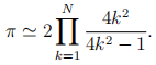
You must do this by writing a function with one input argument N that returns the approximation to π. Outside this function you should set the value of N = 10000, call the function, and print both N and the approximation to π and some short text (string) explaining what is being printed. [16]

h) Below is Python code to perform a grid search for the optimal value of parameter alpha. The code executes without error, but it is incorrect. Explain what is incorrect and explain what should be done to correct the problem.

import numpy as np

from sklearn.neural_network import MLPRegressor

from sklearn.model_selection import train_test_split

from sklearn.model_selection import cross_val_score

from sklearn.datasets import load_boston

# load data

X, y = load_boston(return_X_y=True)

# train-test split

X_train, X_test, y_train, y_test = train_test_split(X,y,random_state=12345)

# initialise variable to find best hyperparameter alpha

max_score = -100

best_alpha = 0

# Everything above this line is correct

for k in range(1,8):

alpha = 10**-k

regr = MLPRegressor(hidden_layer_sizes=(32), alpha=alpha,

    learning_rate_init=0.01, max_iter=5000)

regr.fit(X_train, y_train)

y_predict = regr.predict(X_test)

score = np.linalg.norm(y_predict - y_test)

if score > max_score:

max_score = score

best_alpha = alpha

print("best value for alpha is", best_alpha) 

[16]

2. a) Let f(x) be a smooth function. Using Taylor series, show that the approxima-tion

is a first-order approximation to the first derivative of f. [15]

b) Consider the following Python code meant to generate N samples from the normal distribution with mean zero and variance T.

# Generate N samples from the normal distribution

# with mean zero and variance T.

import numpy as np

rg = np.random.default_rng(12345)

T = 5

N = 1000

X = rg.normal(0,T,N)

Identify the mistake and correct the mistake by rewriting the necessary line or lines of Python. [10]

c) Consider an asset St to follow geometric Brownian motion

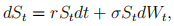
where the risk-free interest rate r and volatility σ are constants. The initial condition is S0. Time t is measured in years.

Consider a trading strategy of purchasing and selling options to produce a dis-counted payoff function given by

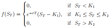
where ST is the value of the asset at expiry T > 0, and K1 and K2 are strike prices satisfying K1 < K2.

(i) State an algorithm for pricing such an option using Monte Carlo simulations with importance sampling for variance reduction. If you wish you may state your algorithm in the form of Python code. You may assume in your algorithm that a method exists to compute , where Φ is the cumulative distribution of the standard normal distribution. [35]

(ii) Suppose one wants to compute the Greek , where V is the option value. Which of the following three methods could be used and which cannot be used?

Finite-difference with path recycling.

Pathwise derivative.

Likelihood ratio.

You do not need to state algorithms, but you do need to justify your an-swers. [20]

d) Suppose we want to estimate the integral

using Monte-Carlo integration with antithetic variance reduction. Suppose that f(y) is such that f(1−y) = 2αy−f(y), for some α > 0. Determine the variance of the integral with antithetic variance reduction. You do not need to determine the variance without variance reduction. 

[20]

3. a) In machine learning we frequently need to scale the feature data. Explain why we scale the training data after performing a train-test split of the full dataset. Explain how we scale test data. 

[20]

b) Consider the following primal constrained minimisation problem

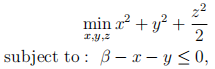
where β > 0 is a constant parameter.

(i) Write the Lagrangian for this problem.

(ii) From this derive the dual problem.

(iii) Solve the dual problem to obtain the solution.

(iv) What is the dimension (number of unknowns) for the primal problem and for the dual problem? For a Support Vector Machine, what is the dimension of the primal and dual problems in terms of number of features and number of examples in the dataset? 

[40]

c) Consider the very simple multilayer perceptron consisting of one input neuron, one output neuron, and two hidden layers with one neuron each.

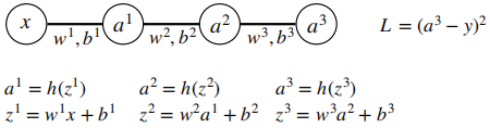
The fitting parameters are . h is the activation function, whose derivative is denoted h'.

Consider a single training pair x, y. The input neuron has activation x and the loss function is 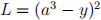. Using back propagation, find

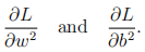
You should express your answers in terms of the fitting parameters and h'.

Let h be the ReLU activation function. Simplify both the above derivatives in the cases

(i) Hidden-layer 1 is not active ( < 0), but other neurons are ( , > 0).

(ii) Output layer is not active ( < 0), but other neurons are ( , > 0). 

[40]