Intro. Modern Ctrl. Eng.                                                    ME 621                                                            L. Wang

Simulation Lab

Due: 5/4/2021, Tuesday, 6:30 pm

Overall Objectives    

In this simulation lab, we will use tools within Matlab to closely study the plant described in Figure 1 and to investigate controllers that assist achieving certain performance.

In Figure 1, each of the carts is supported by frictionless and massless wheels such that both carts can be only slide one single axis. We assume that both carts are sufficiently apart from each other, thereby no collision or contact forces are considered. The only interaction forces between the two carts are the spring and damper forces.

Please note that, for convenience, (i) the two output variables, y1 and y2, are absolute positions; AND (ii) they are offsetted from their equilibrium positions (when no spring forces). As follows, you will complete three parts and document your discoveries:

Part I   review and inspect an implementation of the plant using Matlab Simulink Simscape Multi-body

Part II   derive the state-space representation, implement the plant using. Matlab Simulink State-Space Block, and verify the simulation results with Part I.

Part III   consider y1 as the output, design a PID controller that satisfies certain tracking perfor-mance.

Part IV   consider y1 and y2 as the outputs respectively, design state-feedback controllers using pole placement method such that the controller satisfies certain tracking performance.

Part I                         

Download a startup Simulink model using this link, and you should be able to run it in Matlab.

If you open it in Simulink, you should see the following figure.

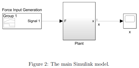
If you open the sub-system (named Plant) and the signal builder block (named Force Input Generation), you should see Figure 3 and Figure 4, respectively.

Task I.1

As illustrated in Figure 3, please inspect the sub-system of the plant using Simscape Multibody closely, element by element (more details about Simscape Multibody), and answer the following questions in your report.

(1) What do the three blocks on the far left do?

(2) Why do we need Rigid Transform 1 and Rigid Transform 2 ? What happens if we don’t have them? Please explain.

(3) Do we need Rigid Transform 3 ? What happens if we don’t have it?

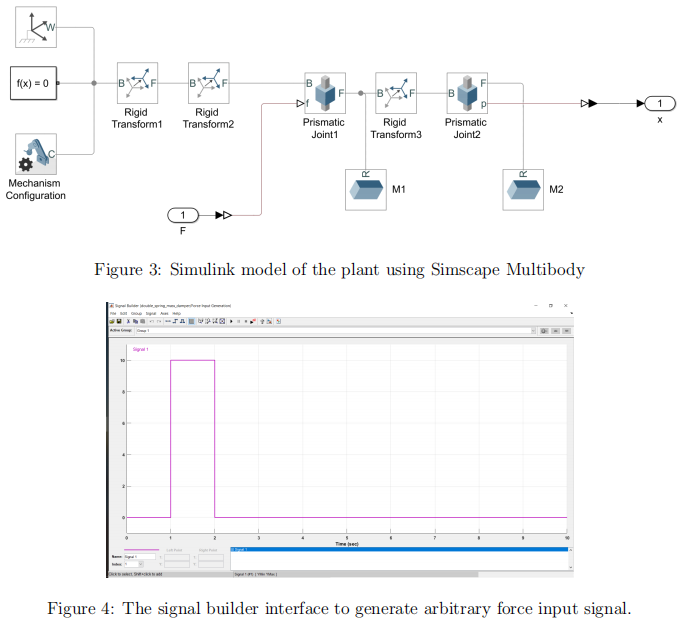
(4) When we run the simulation, we see the spring and damper behaviors of the system. Where are the springs and dampers in the model? How to change the parameters (spring stiffness and damping coefficient)?

(5) Where are the mass properties? How to change them?

Task I.2

Run the simulation, and obtain the system response for 12 seconds given the force input as shown in Figure 4. Save the response using the Simulink scope, in the formats of both figure and data matrices in Matlab workspace.

Task I.3

Modified the plant following Figure 5 by adding a spring-damper couple (the block can be found in the library by searching “spring and damper force”).

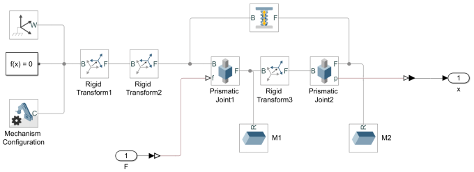
Figure 5: Simulink model of the plant using Simscape Multibody with extra spring and damper.

How would you modify Figure 1 to reflect this change?

Part II                        

In this part, derive the state-space representation for the plant. Obtain the parameter values (mass, spring stiffness, and damping coefficients) from the Simscape Multibody model. Add a state-space block in the original model, as shown in Figure 6.

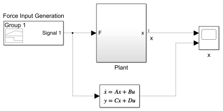
Figure 6: Simulink model of the plant using Simscape Multibody with extra spring and damper.

Task II.1   Derive the state-space representation. Please write detailed derivation steps in your lab report.

Task II.2   Obtain the parameter values (mass, spring stiffness, and damping coefficients). Please document where you find these values explicitly.

Task II.3   Verify that you get the same system response by comparing the two response signals (cart positions) for 12 seconds. Please attach the plots of system response, and explain the plots.

Part III                      

In this part, we consider y1 as the system output and the force u1 as the system input. In addition, when designing the PID controller, let us consider the interaction force between m1 and m2 an unknown disturbance vptq. The PID control law states:

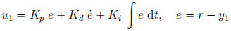
where rptq is the reference.

Task III.1   Let us first assume Ki = 0. How do you choose the values of Kp and Kd such that

– the system is critically damped

– when considering a step reference signal (e.g. r “ 0.1), the steady error is 10%

Verify the PD controller in Simulink model, using the reference as rptq “ 0.1, and report your discovery by plotting the errors for a time period of 100 seconds. Hint: the system step response should be different because the disturbance vptq was not suppose to be included in your differential equation when analyzing the PD gains.

Task III.2   In this task, let us choose the reference as rptq “ 0.1 t. Observe what the steady error is when using the same PD gains?

While keeping the PD gains as the same as above, choose a Ki to reduce the steady error. Verify the PID controller using the reference as rptq “ 0.1 t. Report your discovery by considering the following questions:

– Comment on how different value choices of Ki influence the steady state error.

– Is the system still critically damped?

– If not, how close are the new poles compared to critical damping?

– Comment on how different values choices of Ki affect the poles of the system.

Task III.3   Changing the reference to

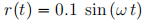
Observe the tracking performances using both the PD and PID controller that you have developed above. Varying the command reference frequency for the following conditions, and report your discovery.

– 0.1 Hz, 0.5 Hz, 1 Hz, 5 Hz, 10 Hz

Draw the Bode plot of the system closed-loop transfer function, what is the cutoff frequency, and relay it to what you discover in simulations.

Part IV                       

In this part, we will use state-feedback controllers in the following format:

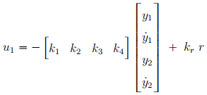
Task IV.1   Consider y1 as the system output and rptq “ 0.1. Pick the poles within the s-plane region such that

– Damping ratio is greater than 0.707

– The imaginary parts are lower than 70

– The settling time of each pole is smaller than 0.1 seconds

Using the selected poles, determine the values for k1, k2, k3, k4, kr. Implement the controller and report your discovery in simulations.

Task IV.2   Consider y2 as the system output and everything else is the same as above.