STAT 441, Final Examination, April 27, 2021

Be reminded that during the exam there is not to be any communication with anybody else about the examination and internet is to be used only to view questions and submit the answers. Give short reasoning for everything you conclude here; if R is required, give the transcript of the code. This exam has 5 problems spanning 4 pages. Good luck!

1. We address the general problem, to be answered in the series of particular questions asked below: whether the classification via the (generalized linear) logistic regression depends on the labeling.

(a) Some R experiments first. Take the good old dataset about riding mowers – it is still sitting out there on eClass, and you can take it also from here:

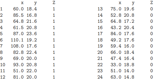
For simplicity, the variables/classifiers will be called now just xi and yi ; the labels will be Zi. (Make sure you make appropriate changes before you continue, and also that you get the dataset in R right.) 

Create a new dataset with the same xi and yi , but with labels  that are opposite to Zi : if Zi = 1 then  = 0, and if Zi = 0 then  = 1. Run logistic regression for both datasets: in the anticipation of what follows in this question, it may be prudent to look at various results that come out of that; but right now, answer only the following question (and nothing else): is there any relationship between the classification predictions obtained for the first (that with Zi) and for the second dataset (that with )? Justify your answer by the transcript of the R output.

(b) Leave R now; what follows is the mathematical part. If the linear parts of the generalized linear model for the dataset with Zi and for the dataset with  are denoted respectively as

what is then the relationship between a, b, c, and – as suggested by the definition of the logistic regression within the generalized linear model? How does this relationship support your empirical finding from (a), if it does at all? The mathematical reasoning here has to be precise and sound, no vague generalities.

2. This is a purely mathematical problem, and the solution is not very long, if you use efficient matrix formalism. Let Y be a n × p usual data matrix, and let S be the (sample) variance-covariance matrix of Y . (You may consider the variables Y centered, that is, the columns of Y summing to 0, if you feel it may be of any help.)

(a) Recall how S is used to compute all principal components – those projections of the datapoints in Y to the pertinent directions – and write it down.

(b) Using the answer you put together in (a), calculate the (sample) variance-covariance matrix of the principal components. What kind of a matrix is it? What does it say about individual principal components?

3. The left panel of the picture below shows a dataset; it is extremely reduced and simplified for the purposes of this exam. As you can see, there are 8 points, labeled 1 to 8; points numbered 1, 5, 7, 8 are black, the remaining ones are white.

There are two variables that serve as classifiers: x and y. The points are classified as “black” or “white” – so these are the labels. The method is k nearest neighbors. The data are already scaled and all that; you may have also noticed that the plot is equiscaled. The distances thus should be apparent; nevertheless, should your eyes give you any doubts, the (rounded) Euclidean distances between the datapoints are shown under the two picture panels.

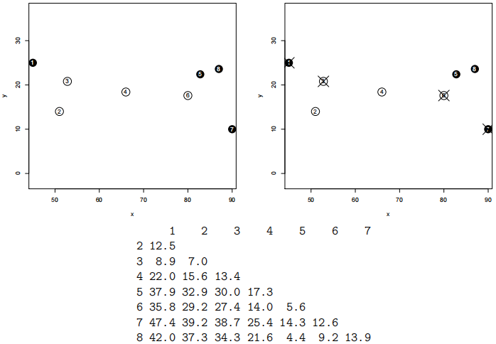
(a) Consider k = 3; that is, the classification method will be 3 nearest neighbors. What is the apparent error rate of this method for the data shown above?

(b) Considering still k = 3, estimate the error rate now by 2-fold crossvalidation. To circumvent any ambiguities introduced by randomness, consider the two “folds” already given: they are indicated, via crossing by X, in the right panel of the picture above. One of the folds thus contains points numbered 1, 3, 6, 7; the other one contains the remaining ones; both contain two black and two white points.

(c) What does the comparison of both methods of estimating an error rate, the method used in (a) and the method used in (b), say? For which k (in the method of k nearest neighbors) it would be even more transparent?

This is a problem to be solved completely by hand, no R tricks (unless you are unable to divide by small numbers without a calculator).

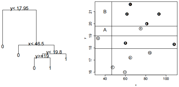
4. The right panel below shows yet another extremely reduced and simplified dataset, with 12 points numbered 1 to 12; those with numbers 1 to 6 labeled as black, those with numbers 7 to 12. There are again two variables serving as classifiers, x and y, and classification is done into the categories “black” and “white”.

(a) The left panel below shows a classification tree constructed out of the dataset; the right panel shows also all the partitioning boundaries involved in the tree. The questions here are actually two: how the tree classifies the point labeled in the right panel as A? And how does it classify the point labeled there as B? Some justification of your answers required, so that they do not appear like mere results of the flips of a coin.

(b) What is intended to be done now is more sophisticated: the repeated construction of a tree-based classifier from the resampled dataset, the method known as bagging. Some 50 or 100 bootstrap samples will be generated; for the purpose of the exam, let us consider only one of those – the code below shows the numbers that were sampled (and thus also reveals the numbers of points that were not sampled; they can be seen crossed by X) on the right panel below):

> ss=sort(sample(1:12,12,replace=TRUE))

> ss

   [1]    2    2    3    4    4    6    7    9    9    10    12    12

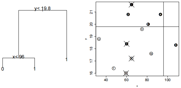
What is the missclassification error rate of the so-called out-of-bag points for this particular bootstrap sample? The justification this time does not have to be so detailed if the result is correct.

5. As shown in many lectures, the R call for the Sammon mapping, a method that gave us a two-dimensional plot of the data with higher dimension, was

> plot(sammon(dist(dataset))$points)

We know that the Sammon mapping has to do something with the quantity

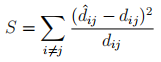
(a) Answer the following questions related to the Sammon mapping method. What are and dij? Which one of those can be seen on the plot? How is the quantity S used in the method?

(b) Based on your answer in (a): if dataset is formed out of the classifiers in the datasets used above, that is, containing only two variables xand y – what is the result supposed to be? Give some reasoning for your answer.