Finance 6318 Professor Day Financial Modeling Spring 2019 Homework Set 3
The following problems are adapted from Introductory Econometrics for Finance by Chris Brooks. Your solutions should be submitted as a Word Document into which you have either typed or pasted a copy of any Excel results or any R code that you have used to generate your results, along with any verbal discussion that is required to explain your results. The assignment should be submitted using the Assignments Link for Homework Assignment 3
1. Assume that you have estimated the following AR(2) model for an economic time series:

where ut is a white noise process. Check the estimated model for stationarity using the characteristic equation. [Hint: Express the model using lag operator notation, take the terms in y to the left hand side, and substitute powers of z for the respective lag operators. Then use the quadratic formula.]
2. Consider the following estimates for the autocorrelations and partial autocorrelations for a
sample of 100 observations for an economic time series:
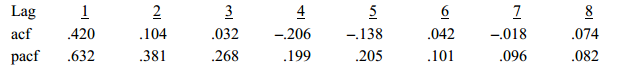 a. Use the estimated autocorrelation and partial autocorrelation functions above to explain which time series model is the most appropriate times series model for these data.
b. Use the Ljung-Box Q* test to determine whether the first three autocorrelation coefficients are jointly significantly different from zero.
3. Assume you have estimated the following ARMA(1,1) model for an economic time series:

a. Construct forecasts for the time series y for dates t, t+1 and t+2 using the estimated ARMA model.
b. Assuming that the actual values for y at dates t, t+1 and t+2 turn out to be –.032, .961, and .203 compute the (out-of-sample) mean squared error
4. Consider a time series of 200 observations for which you have obtained the following estimates for the log of the estimated residual variance ( log(σˆ 2) ):
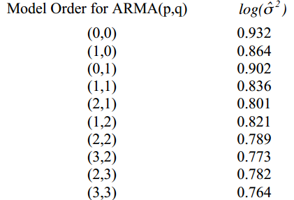
Assuming that a model order greater than (3,3) can be ruled out a priori, determine the optimal order for the model using both the Akaike information criteria and Schwarz’s Bayesian information criteria.
5. Use the pdfetch package for R to download the time series for quarterly Real Gross Domestic Product from the St. Louis Federal Reserve Bank. The field identifier for this time series is GDPC1 and the appropriate R command for download the data is “pdfetch(c(“GDPC1”))”.
a. Estimate a suitable time series model for quarterly GDP, being sure to provide a brief discussion of the criteria that you used for model identification (acf, pacf, and Akaike information criteria). Be sure to present the estimates of your model and if possible perform a joint significance test for the coefficients of your model.
b. Use the time series model that you estimated in part (a) to create a forecast for first quarter (January to March) and second quarter (April to June) Real Gross Disposable Product.
2019-04-05