Economics 360                                                                      Winter 2020-21

Labour Economics                                                               Florian Hoffmann

TAKE-HOME FINAL EXAMINATION

Start:                      Wednesday, April 14th 2021, at 10:00 am, Pacific Time.

Duration:                36 hours

Hand in by:             Thursday, April 15th 2021, 10:00 pm, Pacific Time.

General Instructions (PLEASE READ CAREFULLY!!!):

-  You need to submit your answer on Canvas.

-  You may submit your take-home midterm as pdf, word, scanned hand-written, or photographed handwritten files or any other digital file that can be uploaded to Canvas.

-  Write down your name and student number on page 1 of your submitted file.

-  You are not allowed to collaborate with anyone for this final exam. This includes online tutoring services or similar services. Any indications of collaboration with another student in the class will result in a grade of zero. The director of the BA program will be notified as well.

-  I will use the “honor system” for academic integrity. See question 1.

1. To receive a grade on this final exam you need to write down and sign the following statement:

We are taking this exam under unusual and unpleasant circumstances that affect all of us. It is important that this exam is fair to all students, and that no student has an unfair advantage. With that in mind, I pledge to uphold the highest standards of ethics and academic integrity. I affirm that I have not collaborated with any other student, and that I have not received any help from anyone, including individuals who are not currently enrolled in the course and individuals who o§er help in the internet. All answers are my own.

2. (30 points) Consider the 2-period model of educational choices discussed in class and assume that there are no credit constraints. Use exactly the same notation as in the notes on the model posted on Canvas. Assume that the educational production function is and that the cost function is C (S) = c S. Consider the situation in which the government wants to incentivize individuals to choose high levels of education. To this end, the government uses a policy that pays a subsidy on the direct cost per unit of schooling.

(a) (5 points) Write down the modified cost function that takes the subsidy into account.

(b) (5 points) Derive the schooling level that maximizes the discounted value of "cash-on-hand".

(c) (5 points) Given the optimal level of schooling derived in part (b), write down a mathematical expression for the labor market income earned by an individual in the second period.

(d) (5 points) Suppose there are two individuals whose only difference is that the first individual has a returns-to education parameter A1, while the corresponding value for the second individual is A2. Assume that A2 > A1. Derive the ratio of labor market earnings in period 2 of the two individuals. That is, write down a mathematical expression that has the labor market earnings derived in part(c) of the second individual in the numerator and the corresponding labor market earnings of the first individual in the denominator.

(e) (5 points) Using the ratio derived in (d) as a measure of labor market inequality, how is it affected by the subsidy?

(f) (5 points) Suppose the subsidy is financed by lump-sum taxes on income in period 2. That is, each of the two individuals need to pay exactly the same amount of taxes in period 2 to cover the subsidy. Hence, individual income in period 2 is labor market income minus the tax. How will the tax affect your conclusions about the effect of the subsidy on (after-tax) income inequality? Do you think it will go up or down? You do not need to derive mathematical equations for your answer. A well-reasoned verbal answer is sufficient for this part of the question.

3. (45 points) Last week the government of British Columbia published an official report on the effectiveness of a Universal Basic Income program (UBI) in reducing poverty in British Columbia. The report was written by an expert panel that was chaired by Professor David Green from the Vancouver School of Economics. A central conclusion from the report is that a more effective way than UBI to reduce poverty is to increase accessibility of existing anti-poverty programs.

In this question we use a simple model to investigate how reducing the "time cost" of applying for income maintenance affects labor supply. To this end consider the neoclassical model of labor supply as covered in class and chapters 2 and 3 of the textbook. Assume that individuals have preferences of the form The only source of non-labor income YN are government transfers (i.e. income maintenance programs). Assume that it is time consuming to apply for such transfers. Let t be the time spent on applying and assume that

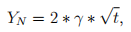
with > 0. That is, if the individual does not spend any time on applying for government transfers it receives none. If it spends an amount t, then the "payoff" is to receive an amount of government transfers of . 

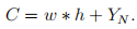
The budget constraint is as usual:

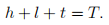
However, the time constraint now needs to take application time into account:

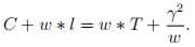
(a) (3 points) Substitute the government transfer equation (1) and the time constraint (3), solved for h, into the budget constraint. Write down the resulting equation.

(b) (2 points) Write down the utility maximization problem subject to the constraint derived in part (a) the individual needs to solve. Notice that this problem will have three instead of two choice variables: C; l; t.

(c) (2 points) Write down the Lagrangian for the problem in (b).

(d) (5 points) Derive the first-order conditions that maximize the Lagrangian in (c). Notice that there will be four instead of three first order conditions. In particular, in addition to taking the derivatives with respect to C; l; you also need to calculate the derivative with respect to t.

(e) (5 points) Using only the first-order condition for t, show that the optimal time spend on applying for government funding is

(f) (5 points) Show that the first-order conditions for consumption and leisure yield exactly the same tangency condition as derived in class.

(g) (5 points) Plugging the solution for derived in part (a) into the first-order condition for the Lagrange multiplier , show that

(h) (10 points) Using the results from (f) and (g), solve for optimal consumption and leisure choices.

(i) (8 points) Suppose the government follows the recommendation of the report and makes existing income maintenance programs more accessible. In our model this can be thought of increasing the returns to the time spent on applications for government funds. That is, assume that the government manages to increase . Analyze the effect of this policy change on consumption and leisure choices. What are your conclusions?

4. (25 points) Describe the various income maintenance programs that we covered in class and discuss their advantages and disadvantages. Use figures with consumption on the  y-axis and leisure on the x-axis to structure your discussion.